Dynamic Programming & Divide and Conquer | Algorithms - Computer Science Engineering (CSE) PDF Download
| Table of contents |
|
| Comparison |
|
| 0-1 Knapsack Problem |
|
| Bellman–Ford Algorithm |
|
| Introduction |
|

Dynamic programming approach is similar to divide and conquer in breaking down the problem into smaller and yet smaller possible sub-problems. But unlike, divide and conquer, these sub-problems are not solved independently. Rather, results of these smaller sub-problems are remembered and used for similar or overlapping sub-problems.
Dynamic programming is used where we have problems, which can be divided into similar sub-problems, so that their results can be re-used. Mostly, these algorithms are used for optimization. Before solving the in-hand sub-problem, dynamic algorithm will try to examine the results of the previously solved sub-problems. The solutions of sub-problems are combined in order to achieve the best solution.
So we can say that −
The problem should be able to be divided into smaller overlapping sub-problem.
An optimum solution can be achieved by using an optimum solution of smaller sub-problems.
Dynamic algorithms use memorization.
Comparison
In contrast to greedy algorithms, where local optimization is addressed, dynamic algorithms are motivated for an overall optimization of the problem.
In contrast to divide and conquer algorithms, where solutions are combined to achieve an overall solution, dynamic algorithms use the output of a smaller sub-problem and then try to optimize a bigger sub-problem. Dynamic algorithms use memorization to remember the output of already solved sub-problems.
Example
The following computer problems can be solved using dynamic programming approach −
- Fibonacci number series
- Knapsack problem
- Tower of Hanoi
- All pair shortest path by Floyd-Warshall
- Shortest path by Dijkstra
- Project scheduling
Dynamic programming can be used in both top-down and bottom-up manner. And of course, most of the times, referring to the previous solution output is cheaper than recomputing in terms of CPU cycles.
0-1 Knapsack Problem
Given weights and values of n items, put these items in a knapsack of capacity W to get the maximum total value in the knapsack. In other words, given two integer arrays val[0..n-1] and wt[0..n-1] which represent values and weights associated with n items respectively. Also given an integer W which represents knapsack capacity, find out the maximum value subset of val[] such that sum of the weights of this subset is smaller than or equal to W. You cannot break an item, either pick the complete item, or don’t pick it (0-1 property).
A simple solution is to consider all subsets of items and calculate the total weight and value of all subsets. Consider the only subsets whose total weight is smaller than W. From all such subsets, pick the maximum value subset.
1) Optimal Substructure:
To consider all subsets of items, there can be two cases for every item: (1) the item is included in the optimal subset, (2) not included in the optimal set.
Therefore, the maximum value that can be obtained from n items is max of following two values.
1) Maximum value obtained by n-1 items and W weight (excluding nth item).
2) Value of nth item plus maximum value obtained by n-1 items and W minus weight of the nth item (including nth item).
If weight of nth item is greater than W, then the nth item cannot be included and case 1 is the only possibility.
2) Overlapping Subproblems
Following is recursive implementation that simply follows the recursive structure mentioned above.
/* A Naive recursive implementation of 0-1 Knapsack problem */
#include<stdio.h>
// A utility function that returns maximum of two integers
int max(int a, int b) { return (a > b)? a : b; }
// Returns the maximum value that can be put in a knapsack of capacity W
int knapSack(int W, int wt[], int val[], int n)
{
// Base Case
if (n == 0 || W == 0)
return 0;
// If weight of the nth item is more than Knapsack capacity W, then
// this item cannot be included in the optimal solution
if (wt[n-1] > W)
return knapSack(W, wt, val, n-1);
// Return the maximum of two cases:
// (1) nth item included
// (2) not included
else return max( val[n-1] + knapSack(W-wt[n-1], wt, val, n-1),
knapSack(W, wt, val, n-1)
);
}
// Driver program to test above function
int main()
{
int val[] = {60, 100, 120};
int wt[] = {10, 20, 30};
int W = 50;
int n = sizeof(val)/sizeof(val[0]);
printf("%d", knapSack(W, wt, val, n));
return 0;
}
Output:
220
It should be noted that the above function computes the same subproblems again and again. See the following recursion tree, K(1, 1) is being evaluated twice. Time complexity of this naive recursive solution is exponential (2^n).
In the following recursion tree, K() refers to knapSack(). The two
parameters indicated in the following recursion tree are n and W.
The recursion tree is for following sample inputs.
wt[] = {1, 1, 1}, W = 2, val[] = {10, 20, 30}
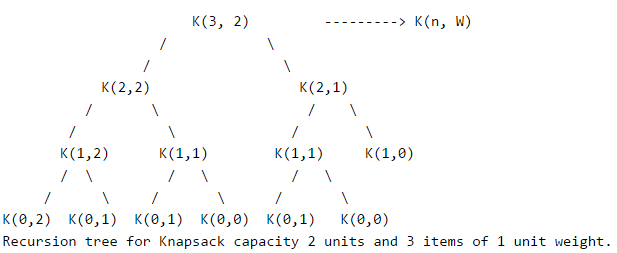
Since suproblems are evaluated again, this problem has Overlapping Subprolems property. So the 0-1 Knapsack problem has both properties of a dynamic programming problem. Like other typical Dynamic programming(DP) problems, recomputations of same subproblems can be avoided by constructing a temporary array K[ ][ ] in bottom up manner. Following is Dynamic Programming based implementation.
// A Dynamic Programming based solution for 0-1 Knapsack problem
#include<stdio.h>
// A utility function that returns maximum of two integers
int max(int a, int b) { return (a > b)? a : b; }
// Returns the maximum value that can be put in a knapsack of capacity W
int knapSack(int W, int wt[], int val[], int n)
{
int i, w;
int K[n+1][W+1];
// Build table K[][] in bottom up manner
for (i = 0; i <= n; i++)
{
for (w = 0; w <= W; w++)
{
if (i==0 || w==0)
K[i][w] = 0;
else if (wt[i-1] <= w)
K[i][w] = max(val[i-1] + K[i-1][w-wt[i-1]], K[i-1][w]);
else
K[i][w] = K[i-1][w];
}
}
return K[n][W];
}
int main()
{
int val[] = {60, 100, 120};
int wt[] = {10, 20, 30};
int W = 50;
int n = sizeof(val)/sizeof(val[0]);
printf("%d", knapSack(W, wt, val, n));
return 0;
}
Output:
220
Time Complexity: O(nW) where n is the number of items and W is the capacity of knapsack.
Bellman–Ford Algorithm
Given a graph and a source vertex src in graph, find shortest paths from src to all vertices in the given graph. The graph may contain negative weight edges.
We have discussed Dijkstra`s algorithm for this problem. Dijksra’s algorithm is a Greedy algorithm and time complexity is O(VLogV) (with the use of Fibonacci heap). Dijkstra doesn’t work for Graphs with negative weight edges, Bellman-Ford works for such graphs. Bellman-Ford is also simpler than Dijkstra and suites well for distributed systems. But time complexity of Bellman-Ford is O(VE), which is more than Dijkstra.
Algorithm
Following are the detailed steps.
Input: Graph and a source vertex src
Output: Shortest distance to all vertices from src. If there is a negative weight cycle, then shortest distances are not calculated, negative weight cycle is reported.
1) This step initializes distances from source to all vertices as infinite and distance to source itself as 0. Create an array dist[] of size |V| with all values as infinite except dist[src] where src is source vertex.
2) This step calculates shortest distances. Do following |V|-1 times where |V| is the number of vertices in given graph.
…..a) Do following for each edge u-v
………………If dist[v] > dist[u] + weight of edge uv, then update dist[v]
………………….dist[v] = dist[u] + weight of edge uv
3) This step reports if there is a negative weight cycle in graph. Do following for each edge u-v
……If dist[v] > dist[u] + weight of edge uv, then “Graph contains negative weight cycle”
The idea of step 3 is, step 2 guarantees shortest distances if graph doesn’t contain negative weight cycle. If we iterate through all edges one more time and get a shorter path for any vertex, then there is a negative weight cycle
How does this work?
Like other Dynamic Programming Problems, the algorithm calculate shortest paths in bottom-up manner. It first calculates the shortest distances for the shortest paths which have at-most one edge in the path. Then, it calculates shortest paths with at-nost 2 edges, and so on. After the ith iteration of outer loop, the shortest paths with at most i edges are calculated. There can be maximum |V| – 1 edges in any simple path, that is why the outer loop runs |v| – 1 times. The idea is, assuming that there is no negative weight cycle, if we have calculated shortest paths with at most i edges, then an iteration over all edges guarantees to give shortest path with at-most (i+1) edges.
Example
Let us understand the algorithm with following example graph.
Let the given source vertex be 0. Initialize all distances as infinite, except the distance to source itself. Total number of vertices in the graph is 5, so all edges must be processed 4 times.
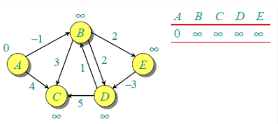
Let all edges are processed in following order: (B,E), (D,B), (B,D), (A,B), (A,C), (D,C), (B,C), (E,D). We get following distances when all edges are processed first time. The first row in shows initial distances. The second row shows distances when edges (B,E), (D,B), (B,D) and (A,B) are processed. The third row shows distances when (A,C) is processed. The fourth row shows when (D,C), (B,C) and (E,D) are processed.
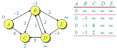
The first iteration guarantees to give all shortest paths which are at most 1 edge long. We get following distances when all edges are processed second time (The last row shows final values).
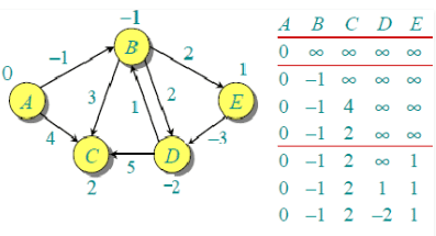
The second iteration guarantees to give all shortest paths which are at most 2 edges long. The algorithm processes all edges 2 more times. The distances are minimized after the second iteration, so third and fourth iterations don’t update the distances.
Implementation:
// A C / C++ program for Bellman-Ford's single source
// shortest path algorithm.
#include <stdio.h>
#include <stdlib.h>
#include <string.h>
#include <limits.h>
// a structure to represent a weighted edge in graph
struct Edge
{
int src, dest, weight;
};
// a structure to represent a connected, directed and
// weighted graph
struct Graph
{
// V-> Number of vertices, E-> Number of edges
int V, E;
// graph is represented as an array of edges.
struct Edge* edge;
};
// Creates a graph with V vertices and E edges
struct Graph* createGraph(int V, int E)
{
struct Graph* graph =
(struct Graph*) malloc( sizeof(struct Graph) );
graph->V = V;
graph->E = E;
graph->edge =
(struct Edge*) malloc( graph->E * sizeof( struct Edge ) );
return graph;
}
// A utility function used to print the solution
void printArr(int dist[], int n)
{
printf("Vertex Distance from Source ");
for (int i = 0; i < n; ++i)
printf("%d %d ", i, dist[i]);
}
// The main function that finds shortest distances from src to
// all other vertices using Bellman-Ford algorithm. The function
// also detects negative weight cycle
void BellmanFord(struct Graph* graph, int src)
{
int V = graph->V;
int E = graph->E;
int dist[V];
// Step 1: Initialize distances from src to all other vertices
// as INFINITE
for (int i = 0; i < V; i++)
dist[i] = INT_MAX;
dist[src] = 0;
// Step 2: Relax all edges |V| - 1 times. A simple shortest
// path from src to any other vertex can have at-most |V| - 1
// edges
for (int i = 1; i <= V-1; i++)
{
for (int j = 0; j < E; j++)
{
int u = graph->edge[j].src;
int v = graph->edge[j].dest;
int weight = graph->edge[j].weight;
if (dist[u] != INT_MAX && dist[u] + weight < dist[v])
dist[v] = dist[u] + weight;
}
}
// Step 3: check for negative-weight cycles. The above step
// guarantees shortest distances if graph doesn't contain
// negative weight cycle. If we get a shorter path, then there
// is a cycle.
for (int i = 0; i < E; i++)
{
int u = graph->edge[i].src;
int v = graph->edge[i].dest;
int weight = graph->edge[i].weight;
if (dist[u] != INT_MAX && dist[u] + weight < dist[v])
printf("Graph contains negative weight cycle");
}
printArr(dist, V);
return;
}
// Driver program to test above functions
int main()
{
/* Let us create the graph given in above example */
int V = 5; // Number of vertices in graph
int E = 8; // Number of edges in graph
struct Graph* graph = createGraph(V, E);
// add edge 0-1 (or A-B in above figure)
graph->edge[0].src = 0;
graph->edge[0].dest = 1;
graph->edge[0].weight = -1;
// add edge 0-2 (or A-C in above figure)
graph->edge[1].src = 0;
graph->edge[1].dest = 2;
graph->edge[1].weight = 4;
// add edge 1-2 (or B-C in above figure)
graph->edge[2].src = 1;
graph->edge[2].dest = 2;
graph->edge[2].weight = 3;
// add edge 1-3 (or B-D in above figure)
graph->edge[3].src = 1;
graph->edge[3].dest = 3;
graph->edge[3].weight = 2;
// add edge 1-4 (or A-E in above figure)
graph->edge[4].src = 1;
graph->edge[4].dest = 4;
graph->edge[4].weight = 2;
// add edge 3-2 (or D-C in above figure)
graph->edge[5].src = 3;
graph->edge[5].dest = 2;
graph->edge[5].weight = 5;
// add edge 3-1 (or D-B in above figure)
graph->edge[6].src = 3;
graph->edge[6].dest = 1;
graph->edge[6].weight = 1;
// add edge 4-3 (or E-D in above figure)
graph->edge[7].src = 4;
graph->edge[7].dest = 3;
graph->edge[7].weight = -3;
BellmanFord(graph, 0);
return 0;
}
Output:
Vertex Distance from Source
0 0
1 -1
2 2
3 -2
4 1
Notes
1) Negative weights are found in various applications of graphs. For example, instead of paying cost for a path, we may get some advantage if we follow the path.
2) Bellman-Ford works better (better than Dijksra’s) for distributed systems. Unlike Dijksra’s where we need to find minimum value of all vertices, in Bellman-Ford, edges are considered one by one.
Exercise
1) The standard Bellman-Ford algorithm reports shortest path only if there is no negative weight cycles. Modify it so that it reports minimum distances even if there is a negative weight cycle.
2) Can we use Dijksra’s algorithm for shortest paths for graphs with negative weights – one idea can be, calculate the minimum weight value, add a positive value (equal to absolute value of minimum weight value) to all weights and run the Dijksra’s algorithm for the modified graph. Will this algorithm work?
Introduction
Like Greedy and Dynamic Programming, Divide and Conquer is an algorithmic paradigm. A typical Divide and Conquer algorithm solves a problem using following three steps.
1. Divide: Break the given problem into subproblems of same type.
2. Conquer: Recursively solve these subproblems
3. Combine: Appropriately combine the answers
Following are some standard algorithms that are Divide and Conquer algorithms.
1) Binary Search is a searching algorithm. In each step, the algorithm compares the input element x with the value of the middle element in array. If the values match, return the index of middle. Otherwise, if x is less than the middle element, then the algorithm recurs for left side of middle element, else recurs for right side of middle element.
2) Quicksort is a sorting algorithm. The algorithm picks a pivot element, rearranges the array elements in such a way that all elements smaller than the picked pivot element move to left side of pivot, and all greater elements move to right side. Finally, the algorithm recursively sorts the subarrays on left and right of pivot element.
3) Merge Sort is also a sorting algorithm. The algorithm divides the array in two halves, recursively sorts them and finally merges the two sorted halves.
4) Closest Pair of Points The problem is to find the closest pair of points in a set of points in x-y plane. The problem can be solved in O(n^2) time by calculating distances of every pair of points and comparing the distances to find the minimum. The Divide and Conquer algorithm solves the problem in O(nLogn) time.
5) Strassen`s Algorithm is an efficient algorithm to multiply two matrices. A simple method to multiply two matrices need 3 nested loops and is O(n^3). Strassen’s algorithm multiplies two matrices in O(n^2.8974) time.
6) Cooley - Tukey Fast Fourier Transform (FFT) algorithm is the most common algorithm for FFT. It is a divide and conquer algorithm which works in O(nlogn) time.
7) Karatsuba algorithm for fast multiplication it does multiplication of two n-digit numbers in at most  single-digit multiplications in general (and exactly
  when n is a power of 2). It is therefore faster than the classical algorithm, which requires n2 single-digit products. If n = 210 = 1024, in particular, the exact counts are 310 = 59,049 and (210)2 = 1,048,576, respectively.
We will publishing above algorithms in separate posts.
Divide and Conquer (D & C) vs Dynamic Programming (DP)
Both paradigms (D & C and DP) divide the given problem into subproblems and solve subproblems. How to choose one of them for a given problem? Divide and Conquer should be used when same subproblems are not evaluated many times. Otherwise Dynamic Programming or Memoization should be used. For example, Binary Search is a Divide and Conquer algorithm, we never evaluate the same subproblems again. On the other hand, for calculating nth Fibonacci number, Dynamic Programming should be preferred.
|
81 videos|113 docs|33 tests
|
FAQs on Dynamic Programming & Divide and Conquer - Algorithms - Computer Science Engineering (CSE)
| 1. What is the difference between Dynamic Programming and Divide and Conquer? |  |
| 2. When should I use Dynamic Programming and when should I use Divide and Conquer? | |
| 3. Can Dynamic Programming and Divide and Conquer be combined? | |
| 4. What are the advantages of using Dynamic Programming and Divide and Conquer? | |
| 5. Are there any limitations or drawbacks of using Dynamic Programming and Divide and Conquer? | |


Objective type Questions
,Sample Paper
,Exam
,Extra Questions
,Dynamic Programming & Divide and Conquer | Algorithms - Computer Science Engineering (CSE)
,Dynamic Programming & Divide and Conquer | Algorithms - Computer Science Engineering (CSE)
,MCQs
,ppt
,Summary
,Important questions
,study material
,Viva Questions
,mock tests for examination
,video lectures
,Dynamic Programming & Divide and Conquer | Algorithms - Computer Science Engineering (CSE)
,Semester Notes
,shortcuts and tricks
,practice quizzes
,past year papers
,Free
,Previous Year Questions with Solutions
;


Dynamic Programming & Divide and Conquer Free PDF Download
Importance of Dynamic Programming & Divide and Conquer
Dynamic Programming & Divide and Conquer Notes
Dynamic Programming & Divide and Conquer Computer Science Engineering (CSE) Questions
Study Dynamic Programming & Divide and Conquer on the App
|
© EduRev
|
Education Revolution
|


|


