Analysis of Loops | Algorithms - Computer Science Engineering (CSE) PDF Download
Analysis of Iterative Programs with Examples
- O(1): Time complexity of a function (or set of statements) is considered as O(1) if it doesn’t contain loop, recursion and call to any other non-constant time function.
// set of non-recursive and non-loop statements
For example swap() function has O(1) time complexity.
A loop or recursion that runs a constant number of times is also considered as O(1). For example the following loop is O(1).
// Here c is a constant
for (int i = 1; i <= c; i++) {
// some O(1) expressions
} - O(n): Time Complexity of a loop is considered as O(n) if the loop variables is incremented / decremented by a constant amount. For example following functions have O(n) time complexity.
// Here c is a positive integer constant
for (int i = 1; i <= n; i += c) {
// some O(1) expressions
}
for (int i = n; i > 0; i -= c) {
// some O(1) expressions
} - O(nc): Time complexity of nested loops is equal to the number of times the innermost statement is executed. For example the following sample loops have O(n2) time complexity
for (int i = 1; i <=n; i += c) {
for (int j = 1; j <=n; j += c) {
// some O(1) expressions
}
}
for (int i = n; i > 0; i -= c) {
for (int j = i+1; j <=n; j += c) {
// some O(1) expressions
}
For example Selection sort and Insertion Sort have O(n2) time complexity. - O(Logn): Time Complexity of a loop is considered as O(Logn) if the loop variables is divided / multiplied by a constant amount.
for (int i = 1; i <=n; i *= c) {
// some O(1) expressions
}
for (int i = n; i > 0; i /= c) {
// some O(1) expressions
}
For example Binary Search(refer iterative implementation) has O(Logn) time complexity. Let us see mathematically how it is O(Log n). The series that we get in first loop is 1, c, c2, c3, … ck. If we put k equals to Logcn, we get cLogcn which is n. - O(LogLogn) Time Complexity of a loop is considered as O(LogLogn) if the loop variables is reduced / increased exponentially by a constant amount.
// Here c is a constant greater than 1
for (int i = 2; i <=n; i = pow(i, c)) {
// some O(1) expressions
}
//Here fun is sqrt or cuberoot or any other constant root
for (int i = n; i > 1; i = fun(i)) {
// some O(1) expressions
}
How to combine time complexities of consecutive loops?
When there are consecutive loops, we calculate time complexity as sum of time complexities of individual loops.
for (int i = 1; i <=m; i += c) {
// some O(1) expressions
}
for (int i = 1; i <=n; i += c) {
// some O(1) expressions
}
Time complexity of above code is O(m) + O(n) which is O(m+n)
If m == n, the time complexity becomes O(2n) which is O(n).
How to calculate time complexity when there are many if, else statements inside loops?
As discussed here, worst case time complexity is the most useful among best, average and worst. Therefore we need to consider worst case. We evaluate the situation when values in if-else conditions cause maximum number of statements to be executed.
For example consider the linear search function where we consider the case when element is present at the end or not present at all.
When the code is too complex to consider all if-else cases, we can get an upper bound by ignoring if else and other complex control statements.
How to calculate time complexity of recursive functions?
Time complexity of a recursive function can be written as a mathematical recurrence relation. To calculate time complexity, we must know how to solve recurrences. We will soon be discussing recurrence solving techniques as a separate post.
Amortized Analysis
Amortized Analysis is used for algorithms where an occasional operation is very slow, but most of the other operations are faster. In Amortized Analysis, we analyze a sequence of operations and guarantee a worst case average time which is lower than the worst case time of a particular expensive operation.
The example data structures whose operations are analyzed using Amortized Analysis are Hash Tables, Disjoint Sets and Splay Trees.
Let us consider an example of a simple hash table insertions. How do we decide table size? There is a trade-off between space and time, if we make hash-table size big, search time becomes slow, but space required becomes high.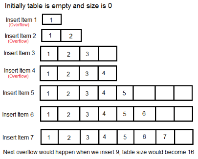
The solution to this trade-off problem is to use Dynamic Table (or Arrays). The idea is to increase size of table whenever it becomes full. Following are the steps to follow when table becomes full.
- Allocate memory for a larger table of size, typically twice the old table.
- Copy the contents of old table to new table.
- Free the old table.
If the table has space available, we simply insert new item in available space.
What is the time complexity of n insertions using the above scheme?
If we use simple analysis, the worst case cost of an insertion is O(n). Therefore, worst case cost of n inserts is n * O(n) which is O(n2). This analysis gives an upper bound, but not a tight upper bound for n insertions as all insertions don’t take Θ(n) time.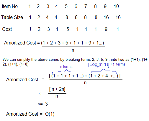
So using Amortized Analysis, we could prove that the Dynamic Table scheme has O(1) insertion time which is a great result used in hashing. Also, the concept of dynamic table is used in vectors in C++, ArrayList in Java.
Following are few important notes:
- Amortized cost of a sequence of operations can be seen as expenses of a salaried person. The average monthly expense of the person is less than or equal to the salary, but the person can spend more money in a particular month by buying a car or something. In other months, he or she saves money for the expensive month.
- The above Amortized Analysis done for Dynamic Array example is called Aggregate Method. There are two more powerful ways to do Amortized analysis called Accounting Method and Potential Method. We will be discussing the other two methods in separate posts.
- The amortized analysis doesn’t involve probability. There is also another different notion of average-case running time where algorithms use randomization to make them faster and expected running time is faster than the worst-case running time. These algorithms are analyzed using Randomized Analysis. Examples of these algorithms are Randomized Quick Sort, Quick Select and Hashing. We will soon be covering Randomized analysis in a different post.
Amortized analysis of insertion in Red-Black Tree
Let us discuss the Amortized Analysis of Red-Black Tree operations (Insertion) using Potential Method.
To perform the amortized analysis of Red-Black Tree Insertion operation, we use Potential(or Physicist’s) method. For potential method, we define a potential function \phi that maps a data structure to a non-negative real value. An operation can result in a change of this potential.
Let us define the potential function \phi in the following manner: (1)
(1)
where n is a node of Red-Black Tree
Potential function  ,over all nodes of the red black tree.
Further, we define the amortized time of an operation as:
Amortized time= 

where h and h’ are the states of Red-Black Tree before and after the operation respectively
c is the actual cost of the operation
The change in potential should be positive for low-cost operations and negative for high-cost operations.
A new node is inserted on a leaf of a red-black tree. We have the leaves of a red-black tree of any one of the following types: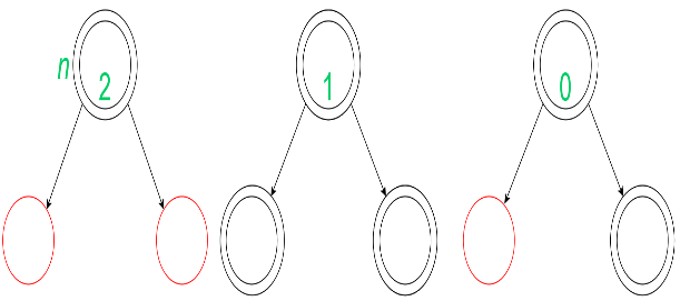
The insertions and their amortized analysis can be represented as:
 This insertion is performed by first recolouring the parent and the other sibling(red). Then the grandparent and uncle of that leaf node is considered for further recolouring which leads to the amortized cost to be -1(when grandparent of the leaf node is red), -2 (when uncle of the leaf is black and grandparent is black) or +1 (when uncle of the leaf is red and grandparent is black). The insertion can be shown as:
 In this insertion, the node is inserted without any changes as the black depth of the leaves remain the same. This is the case when leaf may have a black sibling or do not have any sibling (since we consider the colour of the colour of null node to be black).
So, the amortized cost of this insertion is 0. In this insertion, we cannot recolour the leaf node, its parent and the sibling such that the black depth stays the same as before. So, we need to perform a Left- Left rotation.
After rotation, there are no changes when the grandparent of g(the inserted node) is black. Also, for the case of Red Grandparent of g(the inserted node), we do not have any changes. So, the insertion is completed with amortized cost= +2. The insertion has been depicted below: After calculating these particular amortized costs at the leaf site of a red-black tree we can discuss the nature of total amortized cost of insertion in a red-black tree. Since this may happen that two red nodes may have a parent-child relationship till the root of the red-black tree.
So in extreme(or corner) case, we reduce the number of black nodes with two red children by 1 and we at most increase the number of black nodes with no red children by 1, leaving a net loss of at most 1 to the potential function. Since one unit of potential pays for each operation therefore
Δ ∅ (h) ≤ n
where n is total number of nodes
Thus, the total amortized cost of insertion in Red-Black Tree is O(n).
|
81 videos|80 docs|33 tests
|

|
Explore Courses for Computer Science Engineering (CSE) exam
|

|
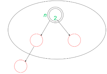 This insertion is performed by first recolouring the parent and the other sibling(red). Then the grandparent and uncle of that leaf node is considered for further recolouring which leads to the amortized cost to be -1(when grandparent of the leaf node is red), -2 (when uncle of the leaf is black and grandparent is black) or +1 (when uncle of the leaf is red and grandparent is black). The insertion can be shown as:
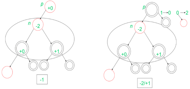
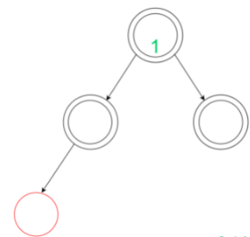 In this insertion, the node is inserted without any changes as the black depth of the leaves remain the same. This is the case when leaf may have a black sibling or do not have any sibling (since we consider the colour of the colour of null node to be black).
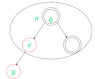 In this insertion, we cannot recolour the leaf node, its parent and the sibling such that the black depth stays the same as before. So, we need to perform a Left- Left rotation.
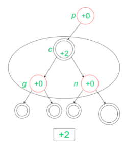 After calculating these particular amortized costs at the leaf site of a red-black tree we can discuss the nature of total amortized cost of insertion in a red-black tree. Since this may happen that two red nodes may have a parent-child relationship till the root of the red-black tree.


