Central Limit Theorem:Example 1 - Mathematical Methods of Physics, UGC - NET Physics | Physics for IIT JAM, UGC - NET, CSIR NET PDF Download

we don't yet have the tools to prove the Central Limit Theorem. And, we won't actually get to proving it until late in Stat 415. It would be good though to get an intuitive feel now for how the CLT works in practice. we'll explore two examples to get a feel for how:
- the skewness (or symmetry!) of the underlying distribution of Xi, and
- the sample size n
affect how well the normal distribution approximates the actual ("exact") distribution of the sample mean  . Well, that's not quite true. We won't actually find the exact distribution of the sample mean in the two examples. We'll instead use simulation to do the work for us. In the first example, we'll take a look at sample means drawn from a symmetric distribution, specifically, the Uniform(0,1) distribution. In the second example, we'll take a look at sample means drawn from a highly skewed distribution, specifically, the chi-square(3) distribution. In each case, we'll see how large the sample size n has to get before the normal distribution does a decent job of approximating the simulated distribution.

Example
Consider taking random samples of various sizes n from the (symmetric) Uniform (0, 1) distribution. At what sample size n does the normal distribution make a good approximation to the actual distribution of the sample mean?
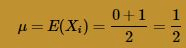
Solution. Our previous work on the continuous Uniform(0, 1) random variable tells us that the mean of a U(0,1) random variable is:
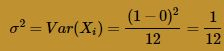
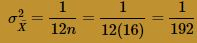
while the variance of a U(0,1) random variable is:
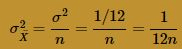
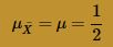
The Central Limit Theorem, therefore, tells us that the sample mean is approximately normally distributed with mean:

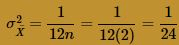
and variance:
Now, our end goal is to compare the normal distribution, as defined by the CLT, to the actual distribution of the sample mean. Now, we could do a lot of theoretical work to find the exact distribution of for various sample sizes n. Instead, we'll use simulation to give us a ballpark idea of the shape of the distribution of . Here's an outline of the general strategy that we'll follow:
- Specify the sample size n.
- Randomly generate 1000 samples of size n from the Uniform (0,1) distribution.
- Use the 1000 generated samples to calculate 1000 sample means from the Uniform (0,1) distribution.
- Create a histogram of the 1000 sample means.
- Compare the histogram to the normal distribution, as defined by the Central Limit Theorem, in order to see how well the Central Limit Theorem works for the given sample size n.
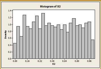
Let's start with a sample size of n = 1. That is, randomly sample 1000 numbers from a Uniform (0,1) distribution, and create a histogram of the 1000 generated numbers. Of course, the histogram should look roughly flat like a Uniform(0,1) distribution. If you're willing to ignore the artifacts of sampling, you can see that our histogram is roughly flat:
Okay, now let's tackle the more interesting sample sizes. Let n = 2. Generating 1000 samples of size n = 2, calculating the 1000 sample means, and creating a histogram of the 1000 sample means, we get:
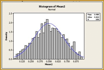
It can actually be shown that the exact distribution of the sample mean of 2 numbers drawn from the Uniform(0, 1) distribution is the triangular distribution. The histogram does look a bit triangular, doesn't it? The blue curve overlaid on the histogram is the normal distribution, as defined by the Central Limit Theorem. That is, the blue curve is the normal distribution with mean:

and variance:
As you can see, already at n = 2, the normal curve wouldn't do too bad of a job of approximating the exact probabilities. Let's increase the sample size to n = 4. Generating 1000 samples of size n = 4, calculating the 1000 sample means, and creating a histogram of the 1000 sample means, we get:
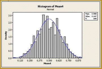
The blue curve overlaid on the histogram is the normal distribution, as defined by the Central Limit Theorem. That is, the blue curve is the normal distribution with mean:
and variance:
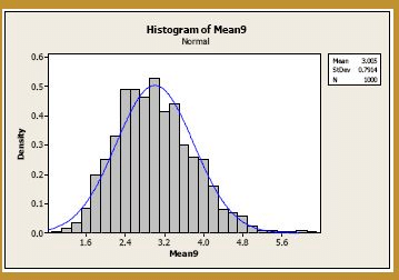
Again, at n = 4, the normal curve does a very good job of approximating the exact probabilities. In fact, it does such a good job, that we could probably stop this exercise already. But let's increase the sample size to n = 9. Generating 1000 samples of size n = 9, calculating the 1000 sample means, and creating a histogram of the 1000 sample means, we get:
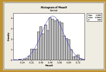
The blue curve overlaid on the histogram is the normal distribution, as defined by the Central Limit Theorem. That is, the blue curve is the normal distribution with mean:

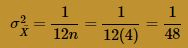
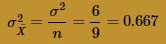
and variance :
And not surprisingly, at n = 9, the normal curve does a very good job of approximating the exact probabilities. There is another interesting thing worth noting though, too. As you can see, as the sample size increases, the variance of the sample mean decreases. That's a good thing, as it doesn't seem that it should be any other way. If you think about it, if it were possible to increase the sample size n to something close to the size of the population, you would expect that the resulting sample means would not vary much, and would be close to the population mean. Of course, the trade-off here is that large sample sizes typically cost lots more money than small sample sizes.
Well, just for the heck of it, let's increase our sample size one more time to n = 16. Generating 1000 samples of size n = 16, calculating the 1000 sample means, and creating a histogram of the 1000 sample means, we get:
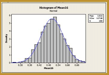
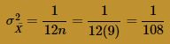
The blue curve overlaid on the histogram is the normal distribution with mean:

and variance:
Again, at n = 16, the normal curve does a very good job of approximating the exact probabilities. Okay, uncle! That's enough of this example! Let's summarize the two take-away messages from this example:
- If the underlying distribution is symmetric, then you don't need a very large sample size for the normal distribution, as defined by the Central Limit Theorem, to do a decent job of approximating the probability distribution of the sample mean.
- The larger the sample size n, the smaller the variance of the sample mean.

Example
Now consider taking random samples of various sizes n from the (skewed) chi-square distribution with 3 degrees of freedom. At what sample size n does the normal distribution make a good approximation to the actual distribution of the sample mean?
Solution. We are going to do exactly what we did in the previous example. The only difference is that our underlying distribution here, that is, the chi-square(3) distribution, is highly-skewed. Now, our previous work on the chi-square distribution tells us that the mean of a chi-square random variable with three degrees of freedom is:
μ=E(Xi)=r=3
while the variance of a chi-square random variable with three degrees of freedom is:
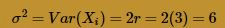
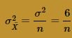
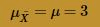
The Central Limit Theorem, therefore, tells us that the sample mean is approximately normally distributed with mean:

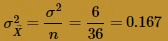
and variance:
Again, we'll follow a strategy similar to that in the above example, namely:
- Specify the sample size n.
- Randomly generate 1000 samples of size n from the chi-square(3) distribution.
- Use the 1000 generated samples to calculate 1000 sample means from the chi-square(3) distribution.
- Create a histogram of the 1000 sample means.
- Compare the histogram to the normal distribution, as defined by the Central Limit Theorem, in order to see how well the Central Limit Theorem works for the given sample size n.
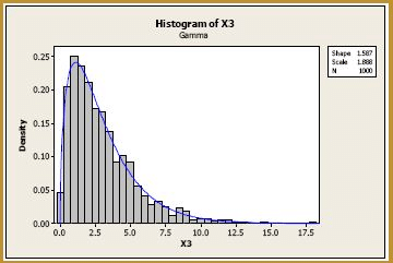
Again, starting with a sample size of n = 1, we randomly sample 1000 numbers from a chi-square(3) distribution, and create a histogram of the 1000 generated numbers. Of course, the histogram should look like a (skewed) chi-square(3) distribution, as the blue curve suggests it does:
Now, let's consider samples of size n = 2. Generating 1000 samples of size n = 2, calculating the 1000 sample means, and creating a histogram of the 1000 sample means, we get:
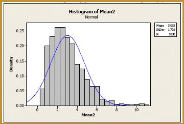
The blue curve overlaid on the histogram is the normal distribution, as defined by the Central Limit Theorem. That is, the blue curve is the normal distribution with mean:

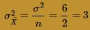
and variance:
As you can see, at n = 2, the normal curve wouldn't do a very job of approximating the exact probabilities. The probability distribution of the sample mean still appears to be quite skewed. Let's increase the sample size to n = 4. Generating 1000 samples of size n = 4, calculating the 1000 sample means, and creating a histogram of the 1000 sample means, we get:
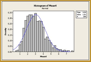
The blue curve overlaid on the histogram is the normal distribution, as defined by the Central Limit Theorem. That is, the blue curve is the normal distribution with mean:

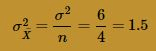
and variance:
Although, at n = 4, the normal curve is doing a better job of approximating the probability distribution of the sample mean, there is still much room for improvement. Let's try n = 9. Generating 1000 samples of size n = 9, calculating the 1000 sample means, and creating a histogram of the 1000 sample means, we get:
The blue curve overlaid on the histogram is the normal distribution, as defined by the Central Limit Theorem. That is, the blue curve is the normal distribution with mean:

and variance:
We're getting closer, but let's really jump up the sample size to, say, n = 25. Generating 1000 samples of size n = 25, calculating the 1000 sample means, and creating a histogram of the 1000 sample means, we get:
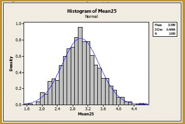
The blue curve overlaid on the histogram is the normal distribution, as defined by the Central Limit Theorem. That is, the blue curve is the normal distribution with mean:

and variance:
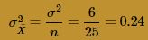
Okay, now we're talking! There's still just a teeny tiny bit of skewness in the sampling distribution. Let's increase the sample size just one more time to, say, n = 36. Generating 1000 samples of size n = 36, calculating the 1000 sample means, and creating a histogram of the 1000 sample means, we get:
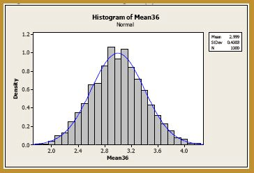
The blue curve overlaid on the histogram is the normal distribution, as defined by the Central Limit Theorem. That is, the blue curve is the normal distribution with mean:
and variance:
Okay, now, I'm perfectly happy! It appears that, at n = 36, the normal curve does a very good job of approximating the exact probabilities. Let's summarize the two take-away messages from this example:
- Again, the larger the sample size n, the smaller the variance of the sample mean. Nothing new there.
- If the underlying distribution is skewed, then you need a larger sample size, typically n > 30, for the normal distribution, as defined by the Central Limit Theorem, to do a decent job of approximating the probability distribution of the sample mean.
FAQs on Central Limit Theorem:Example 1 - Mathematical Methods of Physics, UGC - NET Physics - Physics for IIT JAM, UGC - NET, CSIR NET
| 1. What is the Central Limit Theorem? |  |
| 2. How does the Central Limit Theorem relate to Mathematical Methods of Physics? | |
| 3. Can you explain the concept of the Central Limit Theorem with an example from physics? | |
| 4. How can the Central Limit Theorem be applied in UGC-NET Physics exam? | |
| 5. Are there any limitations or assumptions associated with the Central Limit Theorem? | |


ppt
,Central Limit Theorem:Example 1 - Mathematical Methods of Physics
,study material
,UGC - NET Physics | Physics for IIT JAM
,Exam
,UGC - NET
,CSIR NET
,Important questions
,CSIR NET
,UGC - NET Physics | Physics for IIT JAM
,Central Limit Theorem:Example 1 - Mathematical Methods of Physics
,UGC - NET
,Semester Notes
,mock tests for examination
,Summary
,shortcuts and tricks
,practice quizzes
,Central Limit Theorem:Example 1 - Mathematical Methods of Physics
,Previous Year Questions with Solutions
,Objective type Questions
,MCQs
,video lectures
,UGC - NET Physics | Physics for IIT JAM
,UGC - NET
,Extra Questions
,Sample Paper
,Free
,CSIR NET
,Viva Questions
,past year papers
;


Central Limit Theorem:Example 1 - Mathematical Methods of Physics, UGC - NET Physics Free PDF Download
Importance of Central Limit Theorem:Example 1 - Mathematical Methods of Physics, UGC - NET Physics
Central Limit Theorem:Example 1 - Mathematical Methods of Physics, UGC - NET Physics Notes
Central Limit Theorem:Example 1 - Mathematical Methods of Physics, UGC - NET Physics Physics Questions
Study Central Limit Theorem:Example 1 - Mathematical Methods of Physics, UGC - NET Physics on the App
|
© EduRev
|
Education Revolution
|


|


