Spreadsheet(MS Excel) Chapter Notes | Computer Science for Class 6 PDF Download
Introduction
Microsoft Excel is a powerful spread sheet application that is perfect for maintaining long lists of data, budgets, sales figures and other data. In this chapter you will learn some important and interesting features of Excel like Table, Cell reference, inbuilt functions, sorting of data etc. Let’s discuss these features one by one.
Creating a bar or column chart
To learn how to create a Column and Bar chart in Excel, let's use a simple example of marks secured by some students in Science and Maths that we want to show in a chart format. Note that a column chart is one that presents your data in vertical columns. A bar chart is very similar in terms of the options you have, but presents your data in horizontal bars. The steps below take you through creating a column chart but you can also follow them if you need to create a bar chart.
Preparing chart data
The table below shows the data we want to chart. It is important that your data be presented correctly in order to create a good looking chart. 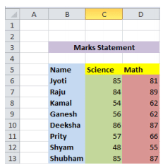
Creating your column chart
Once your data has been prepared correctly, you are ready to create your chart. This is a quick process, but it does involve a number of steps:
- First select your data, making sure that you include all of the data that is to be included in the chart.
- In our example above, that means selecting the range of cells from B5:D13.
- It's important to remember to include the row headings if you want to use those values as axis labels on your finished chart.
- Next, click Insert in the menu. The ribbon will change, and will include a number of chart options(as shown below)

- In our case we are creating a Column chart and Bar chart, so click the Column button first. The following options will then be displayed. As you can see, there are many options available. Select 3D Clustered Column Chart. We can change it to one of the other chart types later if we decide that this one doesn't suit our requirements.
Once you select a chart type, Excel will automatically create the chart and insert it onto your worksheet.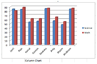
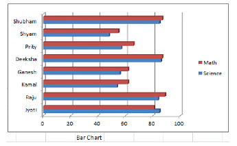
Note the following points about this chart:
- Excel has automatically put labels on an angle to fit neatly into the space available.
- The legend to the right of the chart contains the column heading from our spreadsheet. You can change them by editing the headings in our data table.
- Excel has chosen these colours based on a default theme. You can change the theme if you need to, and the colours will change automatically. You can also override the colours manually if you need to.
- There is no title on the chart by default. You can add one manually, or choose a chart layout that includes one.
Absolute and Relative references in excel formula
You can use three types of cell references in Excel formulas: relative, absolute, and mixed. Using the correct type of cell reference in formulas ensures that they work as expected when you copy them to another location in the worksheet. Formulas and functions are at their most useful when using references, so you need to understand them.
Relative reference: Excel is dynamic when it comes to cell addresses. If you have a cell with a formula that references a different cell's address and you copy the formula from the first cell to another cell, Excel updates the cell reference inside the formula.
Try an example:
- In cell B2, enter 100.
- In cell C2, enter =B2*2.
- Press Enter. And you will see that Cell C2 returns the value 200.
- Now Select cell C2.
- Press Ctrl+C or click the Copy button on the Home tab.
- Click cell C3.
- Press Ctrl+V or click the Paste button on the Home tab.
- If you see a moving marquee around cell C2, press the Esc key.
Cell C3 should be the active cell, but if it is not, just click it once on C3. Look at the Formula bar. The contents of cell C3 are =B3*2, and not the =B2*2 that you copied.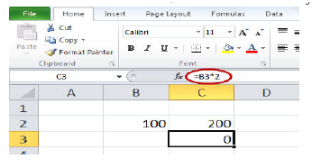
What happened? Excel assumed that if a formula in cell C2 references the cell B2 one cell to the left then the same formula put into cell C3 is supposed to reference cell B3 also one cell to the left. Relative references adjust when you copy a formula.
By default, Excel uses relative reference. Let’s see another example. See the formula in cell D2 below. Cell D2 references (points to) cell B2 and cell C2. Both references are relative.
1. Select cell D2, click on the lower right corner of cell D2 and drag it down to cell D5.
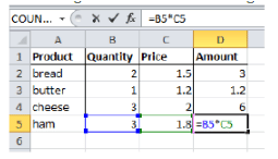
2. Cell D3 references cell B3 and cell C3. Cell D4 references cell B4 and cell C4. Cell D5 references cell B5 and cell C5. In other words: each cell references its two neighbours on the left.
Absolute cell reference: Sometimes you don't want relative addressing but rather absolute addressing: making a cell reference fixed to an absolute cell address so that it doesn't change when the formula is copied. In an absolute cell reference, a dollar sign ($) precedes both the column letter and the row number. See the following example
1. To create an absolute reference to cell H3, place a $ symbol in front of the column letter and row number of cell H3 ($H$3) in the formula of cell E3.
2. Now we can quickly drag this formula to the other cells.
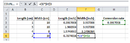
The reference to cell H3 is fixed (when we drag the formula down and across). As a result, the correct lengths and widths in inches are calculated.
Mixed reference: You can also have a mixed reference in which the column is absolute and the row is relative or vice versa. To create a mixed reference, you use the dollar sign in front of just the column letter or row number. Here are some examples:

|
49 videos|20 docs|6 tests
|
FAQs on Spreadsheet(MS Excel) Chapter Notes - Computer Science for Class 6
| 1. What is the importance of using CBSE Class 6 Computer Science Spreadsheet Ms Excel Notes? |  |
| 2. How can CBSE Class 6 Computer Science Spreadsheet Ms Excel Notes be used effectively? |  |
| 3. Are there any additional resources available for CBSE Class 6 Computer Science Spreadsheet Ms Excel Notes? |  |
| 4. How can students create a bar or column chart using Excel as mentioned in the notes? |  |
| 5. What is the difference between relative and absolute cell references in Excel, as discussed in the notes? |  |

|
Explore Courses for Class 6 exam
|

|


