Legendre Special Function - 3 | Physics for IIT JAM, UGC - NET, CSIR NET PDF Download

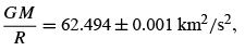
Example 12.3.1 EARTH’S GRAVITATIONAL FIELD 

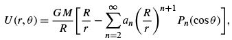
An example of a Legendre series is provided by the description of the Earth’s gravitational potential U (for exterior points), neglecting azimuthal effects. With

R = equatorial radius = 6378.1 ± 0.1km

we write

          (12.52)

a Legendre series. Artificial satellite motions have shown that

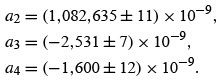
This is the famous pear-shaped deformation of the Earth. Other coefficients have been computed through n = 20. Note that P₁ is omitted because the origin from which r is measured is the Earth’s center of mass ( P₁ would represent a displacement).
More recent satellite data permit a determination of the longitudinal dependence of the Earth’s gravitational field. Such dependence may be described by a Laplace series.

Example 12.3.2 SPHERE IN A UNIFORM FIELD 

Another illustration of the use of Legendre polynomials is provided by the problem of a neutral conducting sphere (radius r₀ ) placed in a (previously) uniform electric field (Fig. 12.8). The problem is to find the new, perturbed, electrostatic potential. If we call the electrostatic potential V , it satisfies

∇² V = 0,                       (12.53)

Laplace’s equation. We select spherical polar coordinates because of the spherical shape of the conductor. (This will simplify the application of the boundary condition at the surface of the conductor.) Separating variables and glancing at Table 9.2, we can write the unknown potential V(r, θ ) in the region outside the sphere as a linear combination of solutions:

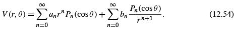
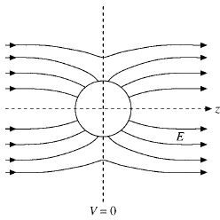
FIGURE 12.8 Conducting sphere in a uniform field.

No ϕ -dependence appears because of the axial symmetry of our problem. (The center of the conducting sphere is taken as the origin and the z-axis is oriented parallel to the original uniform field.) It might be noted here that n is an integer, because only for integral n is the θ dependence well behaved at cos θ =±1. For nonintegral n the solutions of Legendre’s equation diverge at the ends of the interval [−1, 1], the poles θ = 0,π of the sphere. It is for this same reason that the second solution of Legendre’s equation, Q_n , is also excluded.
Now we turn to our (Dirichlet) boundary conditions to determine the unknown an and bn of our series solution, Eq. (12.54). If the original, unperturbed electrostatic field is E₀ , we require, as one boundary condition,

V(r →∞) =−E_0z =−E_0r cos θ =−E_0rP₁(cos θ). (12.55)

Since our Legendre series is unique, we may equate coefficients of P_n (cos θ) in Eq. (12.54) (r →∞) and Eq. (12.55) to obtain

a_n = 0,n > 1 and n = 0,a1 =−E0. (12.56)

If a_n ≠ 0 for n> 1, these terms would dominate at large r and the boundary condition (Eq. (12.55)) could not be satisfied.
As a second boundary condition, we may choose the conducting sphere and the plane θ = π/2 to be at zero potential, which means that Eq. (12.54) now becomes

In order that this may hold for all values of θ , each coefficient of P_n (cos θ) must vanish.¹²

Hence

b₀ = 0,¹³         b_n = 0,            n ≥ 2,                          (12.58)

whereas

           (12.59)

The electrostatic potential (outside the sphere) is then

      (12.60)

it was shown that a solution of Laplace’s equation that satisfied the boundary conditions over the entire boundary was unique. The electrostatic potential V ,asgiven by Eq. (12.60), is a solution of Laplace’s equation. It satisfies our boundary conditions and therefore is the solution of Laplace’s equation for this problem.

It may further be shown that there is an induced surface charge density

        (12.61)

ELECTROSTATIC POTENTIAL OF A RING OF CHARGE 

As a further example, consider the electrostatic potential produced by a conducting ring carrying a total electric charge q (Fig. 12.9). From electrostatics the potential ψ satisfies Laplace’s equation. Separating variables in spherical polar coordinates (compare Table 9.2), we obtain

            (12.63a)

Here a is the radius of the ring that is assumed to be in the θ = π/2 plane. There is no ϕ (azimuthal) dependence because of the cylindrical symmetry of the system. The terms with positive exponent in the radial dependence have been rejected because the potential must have an asymptotic behavior,

              (12.63b)

The problem is to determine the coefficients c_n in Eq. (12.63a). This may be done by evaluating ψ(r, θ ) at θ = 0,r = z, and comparing with an independent calculation of the

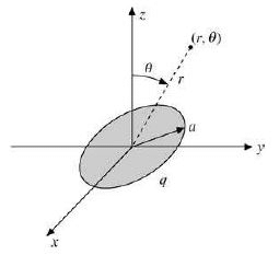
FIGURE 12.9 : Charged, conducting ring.

potential from Coulomb’s law. In effect, we are using a boundary condition along the z - axis. From Coulomb’s law (with all charge equidistant),

The last step uses the result of Exercise 8.1.15. Now, Eq. (12.63a) evaluated at θ = 0,r = z (with P_n (1) = 1), yields

        (12.63d)

Comparing Eqs. (12.63c) and (12.63d), we get c_n = 0 for n odd. Setting n = 2s ,wehave

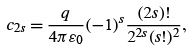             (12.63e)

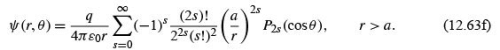
and our electrostatic potential ψ(r, θ ) is given by

The magnetic analog of this problem appears in Example 12.5.3.

ALTERNATE DEFINITIONS OF LEGENDRE POLYNOMIALS

Rodrigues’ Formula

The series form of the Legendre polynomials (Eq. (12.8)) of Section 12.1 may be transformed as follows. From Eq. (12.8),

  (12.64)

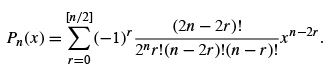
For n an integer,

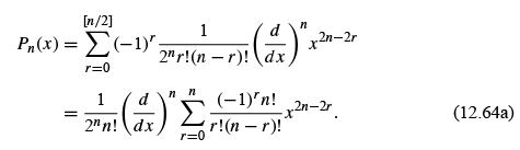
Note the extension of the upper limit. The reader is asked to show in Exercise 12.4.1 that the additional terms [n/2]+ 1to n in the summation contribute nothing. However, the effect of these extra terms is to permit the replacement of the new summation by (x ² − 1)ⁿ (binomial theorem once again) to obtain

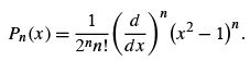            (12.65)

This is Rodrigues’ formula. It is useful in proving many of the properties of the Legendre polynomials, such as orthogonality. The Rodrigues definition is define the associated Legendre functions.  it is used to identify the orbital angular momentum eigenfunctions.

Schlaefli Integral

Rodrigues’ formula provides a means of developing an integral representation of P_n (z). Using Cauchy’s integral formula. 

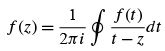       (12.66)

with

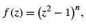       (12.67)

we have

        (12.68)

with the contour enclosing the point t = z

This is the Schlaefli integral. Margenau and Murphy ¹⁴ use this to derive the recurrence relations we obtained from the generating function.
The Schlaefli integral may readily be shown to satisfy Legendre’s equation by differentiation and direct substitution (Fig. 12.11). We obtain

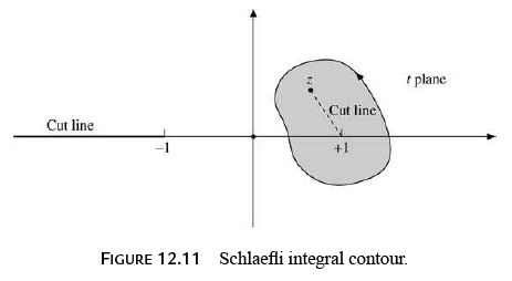
nothing new. A contour about t =+1 and t =−1 will lead to a second solution, Qν (z) .