Probability Distribution | Applied Mathematics for Class 12 - Commerce PDF Download

Introduction

In the  field of Statistics, Probability Distribution plays a major role in giving out the possibility of every outcome pertaining to a random experiment or event. It gives forth the probabilities of various possible occurrences. One is already aware that Probability refers to the measure of the uncertainties found in different phenomenons.
A Probability Distribution is a table or an equation that interconnects each outcome of a statistical experiment with its probability of occurrence.
To understand the concept of a Probability Distribution, it is important to know variables, random variables, and some other notations.
Random experiments are often defined to be the result of an experiment whose result is hard to predict. For instance, while flipping a coin, one cannot predict the outcome, that is, whether it will be a head or a tail. The possible result witnessed in a random experiment is termed as its outcome. While the set of outcomes is referred to as the sample point. With reference to these experiments or events, one can easily create a Probability table in terms of the expected variables and probabilities. 

• Variables:  A variable is defined as any symbol that can take any particular set of values.
• Random Variable: When the value of any variable is the outcome of a statistical experiment, that variable is determined as a Probability Distribution of random variables. It can be Discrete (not constant) or Continuous or both.

Mostly, statisticians make use of capital letters to denote a Probability Distribution of random variables and small-case letters to represent any of its values.
X denotes the Probability Distribution of random variable X
P(X) denotes the Probability of X.
p(X = x) denotes the Probability that random variable x is equivalent to any particular value, represented by X. For example: P (X = 1) states the Probability Distribution of the random variable X is equivalent to 1. 

Probability Distribution of Random Variables

• A random variable is said to have a Probability Distribution that goes on to define the Probability of its unknown values. These random variables can often be Discrete and at other times Continuous, or even both. This refers to the fact that it will take any designated finite or countable values along with a Probability mass Function of the given random variable’s Probability Distribution. It can also take up any numerical value in any given interval or even set of intervals.
• Any two random variables possessing equal Probability Distribution can still vary due to their relationship with other random variables. Random variates is a term used to describe the recognition of the random variable. 

Probability Distribution Definition

• Probability Distributions give up the possible outcome of any random event. It is also identified on the grounds of underlying sample space as a set of possible outcomes of any random experiment. These settings can be a set of Prime Numbers, a set of Real Numbers, a set of Complex Numbers, or a set of any entities. The Probability Distribution is a part of Probability and Statistics.
• Random experiments are termed as the outcomes of an experiment whose results cannot be predicted. For example- if we toss a coin, we cannot predict what will appear, either the head or tail. The possible result of a random experiment is known as the outcome. And the set of outcomes is termed as a sample point. Through these possibilities, we can design a Probability table on the basis of variables and probabilities.

Types of Probability Distribution:

There are two types of Probability Distribution which are used for distinct purposes and various types of data generation processes.

These Two Types of Probability Distribution are:

• Normal or Continuous Probability Distribution
• Binomial or Discrete Probability Distribution

Normal Probability Distribution
In this Distribution, the set of all possible outcomes can take their values on a continuous range. It is also known as Continuous or cumulative Probability Distribution.
For example- Set of real Numbers, set of prime numbers, are the Normal Distribution examples as they provide all possible outcomes of real Numbers and Prime Numbers. Real-life scenarios such as the temperature of a day is an example of Continuous Distribution.
As the Normal Distribution Statistics predict some natural events clearly, it has developed a standard of recommendation for many Probability issues. Some examples are:

• Rolling of a dice
• Tossing a  coin
• Height of a newly born babies
• Size of men or women's shoes.
• Income Distribution of a country between rich and poor

Binomial / Discrete Probability Distribution
The Binomial Distribution is also termed as a Discrete Probability Function where the set of outcomes is Discrete in nature. For example: if a dice is rolled, then all its possible outcomes will be Discrete in nature and it gives the mass of outcome. It is also considered a Probability mass Function

• In a  real-life scenario the concept of Binomial Distribution is used for:
• To find out the number of men and women working in a college
• To find the Number of used and unused particles while manufacturing a product
• To check the Number of people watching the particular channel by calculating the or yes or no.
• To take a survey of positive and negative feedback for some issues.

Negative Binomial Distribution

A negative Binomial Distribution is a term used when in a given Discrete Probability Distribution, before a particularized Number of failures occurs, the Number of the success in the series of the independent and identical Bernoulli trials happens. The Number of failures here is denoted by the letter ‘r’. For example, while throwing a dice,  we determine the occurrence of the Number 1 as a failure and all the mom-1’s as a success. Now, throwing the dice Continuously until the Number 1 occurs three times, indicating three failures, in this case, the Probability Distribution of the non-1 Numbers that have arrived would be referred to as the Negative Binomial Distribution. 

Poisson Probability Distribution

This Discrete Probability Distribution presents the Probability of a given number of events that occur in time and space, at a steady rate. It had gained its name from the French Mathematician Simeon Denis Poisson. This kind of Distribution also finds its relevance in other events occurring at particular intervals, for example, distance, area, and volume. Some examples of these are; 

• Number of patients arriving at the hospital in the time interval 10 to 11 AM
• Number of emails that a manager receives in the office hours. 

PRIOR Probability

Prior Probability, also known as prior, of a quantity that is unpredictable, refers to the Probability Distribution which expresses one’s faith in the given quantity before any given proof is taken into records. For example, the prior Probability Distribution points at the relative proportions of voters that might vote for a given politician at the election. The hidden quantity can point at the possible variable rather than at a perceptible variable. 

Probability Distribution Formulas

Here are some of the Probability Distribution formulas based on their types. 

The Formula for the Normal Distribution

Here,
μ = Mean Value
σ  =Standard Deviation
x = Normal random variable
If mean μ = 0, and standard deviation = 1, then this Distribution is termed as Normal Distribution.
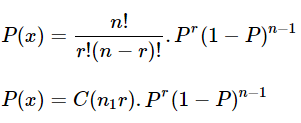
The Formula for the Binomial Distribution

Here,
n=Total Number of events
r= Total Number of successful events
p = successful on a single trial Probability,
1-p =  Failure Probability
ⁿC_r = n!r!(n−r)!

Probability Distribution Function

The Functions which are used to define the Distribution of Probability are termed as a  Probability Distribution Function. These Functions can be defined on the basis of their types. These Probability Distribution Functions are also used in respect of Probability Density Functions for any of the given random variables.

In Normal Distribution, the Function of a real-valued random variable X is the Function derived by:

Fx(x) =P(X ≤ x)

Where P indicates the Probability that the random variable X occurs on less than or equal to the value of  X.

For the closed interval (a →b) the cumulative Probability Function can be identified as:

P( a< X ≤ b) = Fx (b) -Fx(a)

If the cumulative Probability Function is expressed as integral of the Probability density Function fx, then,

In terms of a random variable X= b, cumulative Probability Function can be defined as:

As we know, the Binomial Distribution is determined as the Probability of mass or Discrete random variable which yields exactly some values. This Distribution is also termed Probability mass Distribution and the Function linked with it is known as Probability mass Function.
For example,
A random variable X and sample space S are termed as
X:S  → A
And A ∈ R, where R is termed as a Discrete random variable
Then, Probability mass Function fx : A -
0,1
0,1 or X can be termed as:
Fx (x) = Pr(X = x) = P ({s ∈ S: X(s) = x})

Probability Distribution Table Introduction

The Probability Distribution table is designed in terms of a random variable and possible outcomes. For instance- random variable X is a real-valued function whose domain is considered as the sample space of a random experiment. The Probability Distribution of P(X) of a random variable X is the arrangement of Numbers.
Where Pi > 0 , i = 1 to n and P₁ + P₂ + P₃ ….. P_n = 1

Probability Distribution Table

Where Pi > 0 , i = 1 to n and P₁ + P₂ + P₃ ….. P_n = 1

Solved Example

Example 1: What is the probability of getting 7 heads, if a coin is tossed for 12 times?

Number of trials (n) =12
Number Of success (r) - 7
Probability of single-trial (p)=  ½ = 0.5

ⁿC_r
 =  n!/r! X (n-r)!
=12! /7! (12-7)!
= 12! / 7! 5!
= 95040120
= 792
p^r = 0.5 = 0.0078125

To find(1−p)^(n−r), calculate (1-p) and (n-r)
(1-p) =1-0.5 = 0.5
n-r = 12-7= 5
(1−p)^(n−r) = (0.5)⁽⁷⁾ = 0.03125

Now calculate

P(X = r)(ⁿC_r.p)^r.(1−p)^n−r
= 792 x 0.0078125 x 0.03125
= 0.193359375
Hence, the Probability of getting 7 head is 0.19

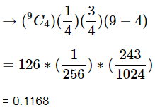
Example 2: The Probability of a man hitting the target is ¼. If he fires 9 times, then find the Probability that he hits the target exactly 4 times.

Total Number of fires (n) = 9
Total Number of success hites = r = 4
Probability of hitting the targets
Probability of not hitting the targets
Calculating ⁿC_r

Probability of the person hits the target exactly 4 times