Short Answer Type Questions
Q1: What are two alternative ways of determining equilibrium level of income ? How are these related ?
Ans: Two alternative ways of determining equilibrium level of income are :
(i) Aggregate Demand - Aggregate Supply Approach (AD-AS Approach) 1
(ii) Saving-Investment Approach (S-I Approach).
Interrelation between the two approaches : AD = AS (AD-AS Approach) C + I = C + S
I = S (S-I approach)
Q2: An economy is in equilibrium. Calculate the Marginal Propensity to Save from the following : National Income = 1,000 Autonomous Consumption = 100 Investment= 120
Ans: Given, Y = 1,000
C = 100
I = 120
Calculate MPS = ?
We known, Y = C + b(Y) + I
or 1,000 = 100 + b(1,000) + 120
or 1,000 = 220 + 1,000b
or b = 1000 - 220/1000
b = 780/1000
or b = 0.78
∴ 1 – MPC = MPS
or 1 – 0.78 = MPS
or MPS = 0.22
Q3: Calculate Marginal Propensity to Consume from the following data about an economy which is in equilibrium:
National Income = 1,500
Autonomous Consumption Expenditure = 300 Investment Expenditure = 300
Ans: Y = C + I
and C = C +b(Y)
∴ Y = C + b(Y) + I
or 1,500 = 300 + (b)1,500 + 300
or 1,500 – b(1,500) = 300 + 300
or 1,500 (b) = 1,500 – 600 1½
or 1,500 (b) = 900
or (b) = 900/1500 = 0.6
∴ b or (MPC) = 0.6
Q4: What is ex-Ante consumption? Distinguish between autonomous consumption and induced consumption
Ans: Ex-ante consumption refers to the consumption expenditure planned to be incurred during a period.
Autonomous Consumption refers to the consumption expenditure which does not depend upon the level of income, i.e. the consumption at zero level of income.
Whereas, Induced Consumption expenditure is directly determined by the level of income.
Q5: Calculate equilibrium level of income : (i) Autonomous consumption = 200 (ii) Marginal propensity to consume = 0.9 (iii) Investment expenditure = 1,000A
Ans: Y = C + I and C = 200 + 0.9
Y; I = 1,000 Y = 200 + 0.9Y + 1,000
⇒ 0.1Y = 1,200 Y = 12,000
Q6: An economy is in equilibrium. From the following data calculate investment expenditure :
(i) Marginal propensity to consume = 0·9
(ii) Autonomous consumption = 200
(iii) Level of income = 10000
Ans: Y = C + I ½
= C + MPC(Y) + I 1½
10,000 = 200 + 9/10((10,000) + I
= 10,000 – 200 – 9,000 = 800
Q7: Calculate Autonomous Consumption Expen- diture from the following data about an economy which is in equilibrium : National Income = 900
Marginal Propensity to Save = 0.10 Investment Expenditure = 80
Ans: Y = C + I
and C = C + b(Y)
or Y = C + b(Y) + I 1½
∴ MPC = (1 – MPS) \ (1 – 0.1) = 0.9
900 = C + 0.9 (900) + 80 1½
or 900 = C + 810 + 80
or C = 900 – 890
or C = 10
Q8: Calculate “Investment Expenditure” from the following data about an economy which is in equilibrium :
National Income = 700
Marginal Propensity to Consume = 0.8 Autonomous Consumption Expenditure = 70
Ans: Y = C + I
We know, C = C + b(Y)
∴ Y = C + b(Y) + I 1½
MPC + MPS = 1 \ MPC = 1 – MPS
∴ MPC = 1 – 0.2
= 0.8
∴ 1,000 = 100 + (0.8) (1,000) + I 1½
or 1,000 = 100 + 800 + I
Q9: An economy is in equilibrium. Find ‘autonomous consumption’ from the following : National Income= 1,000 Marginal Propensity to Consume = 0.8 Investment Expenditure= 100
Ans: Given, Y = 1,000, MPC = 0.8, I = 100
C = ?
We known,
Y = C + b(Y) + I
or 1,000 = C + 0.8(1,000) + 100
or 1,000 = C + 800 + 100
or C = 1,000 – 900
or C = 100
or I = 1,000 – 900
or I = 100
Q10: S = – 100 + 0.2 Y is the saving function in an economy. Investment expenditure is 5,000. Calculate the equilibrium level of income.
Ans: S = –100 + 0.2y
At equilibrium S = I
I = 5,000
∴ 5,000 = –100 + 0.2y
0.2y = 5,100
y = 25,500
Q11: An economy is in equilibrium. Find Marginal Propensity to Consume from the following : National Income= 2,000 Autonomous Consumption = 400 Investment Expenditure=200
Ans: Given, Y = 2,000, C = 400, I = 200
Find out MPC = ? We known, Y = C + b(Y) + I
or 2,000 = 400 + b(2,000) + 200
or 2,000 = 400 + 200 + b(2,000)
or 2,000 – 600 = b(2,000)
or b = 1400/2000 = 0.7
∴ b or MPC = 0.7
Q12: An economy is in equilibrium. Calculate the Investment Expenditure from the following : National Income = 800 Marginal Propensity to Save = 0.3 Autonomous Consumption = 100
Ans: Given, Y = 800 MPS = 0.3
or MPC = 1 – MPS = 1 – 0.3 = 0.7 C = 100 We known, Y = C + b(Y) + I
or 800 = 100 + 0.7 (800) + I
or 800 = 100 + 560 + I or I = 800 – 660 or I = 140
Q13: Calculate “Investment Expenditure” from the following data about an economy which is in equilibrium :
National Income = 700
Marginal Propensity to Consume = 0.8 Autonomous Consumption Expenditure = 70
Ans: Y = C + I
We know, C = C + b(Y)
or Y = C + b(Y) + I 1½
700 = 70 + 0.8 (700) + I 1½
or 700 = 70 + 560 + I
or I = 700 – 630
or I = 70
Q14: Calculate Marginal Propensity to Consume from the following data about an economy which is in equilibrium :
National Income = 2,000
Autonomous Consumption Expenditure = 200 Investment Expenditure = 100
Ans: Y = C + I
We know, C = C + b(Y)
∴ Y = C + b(Y) + I 1½
or 2,000 = 200 + b(2,000) + 100 1½
or 2,000 – 300 = 2,000 b
or 2,000 b = 1,700
b = 1700/2000 = 0.85
b = 0.85
Q15: Shouldn’t greater saving imply greater investment and greater flow of goods and services?
Ans: Greater Saving implies greater investment and greater flow of goods and services in poor economies where aggregate supply is lacking in relation to aggregate demand. But this relationship doesn’t hold good in case of affluent economies where aggregate demand lacks in relation to aggregate demand. In these economies, greater savings would mean lesser comsumption, resulting in lesser demand and lesser production even when capacity produce exists in the economy.
Long Answer Type Questions
Q1: Explain the Consumption Function and Saving Function.
Ans: Consumption Function—The relationship between the consumption expenditure and the income is known as Consumption Function.
C = f(Y)
Where C = Consumption Expenditure
f = Function
Y = Income Algebraic Expression of Consumption Function—
The algebraic expression of Consumption Function is given by :
C = C + b(Y)
Here, C = Consumption Expenditure
C = Minimum Level of Consumption at zero income
b = Marginal Propensity to consume
Y = Income
It is of two types :
(i) Average Propensity to Consume (APC) : The ratio between the consumption expenditure and income is called Average Propensity to Consume.
APC = C/Y
(ii) Marginal Propensity to Consume (MPC) :The ratio between the change in consumption expenditure to change in income is called Marginal Propensity to Consume.
MPC = ΔC/ΔY
Saving Function :The relationship between saving and income is known as Saving Function.
S = f(Y)
Saving is the residual of income after consumption.
S = Y – C
Algebraic Expression of Saving Function : It is given by
S = (–) S + b(Y)
Here, S = Saving
S– = Minimum level of Saving at zero income i.e. negative savings b = Marginal Propensity to save Y = Income
It is of two types :
(i) Average Propensity to Save (APS) : The ratio between total saving and the total income in an economy at a given level of income is termed as Average Propensity to Save (APS).
APS = S/Y
(ii) Marginal Propensity to Save (MPS) : The ratio between the change in saving to the change in income is known as Marginal Propensity to Save.
MPS = ΔS/ΔY
Q2: Given Saving Curve, derive Consumption Curve and state the steps in doing so. Use diagram.
OR
Outline the steps required to be taken in deriving the consumption curve from given saving curve. Use diagram.
Ans: Given Saving Curve SS’
(i) Draw a 45º line from the origin.
(ii) Take OC equal to OS on the Y-axis.
(iii) Draw a perpendicular line from B to B’ on OX-axis which intersect 45º line at point B.
(iv) Join C and B and extend it to get consumption curve CC’.
Q3: Given Consumption Curve, derive Saving Curve and state the steps taken in the process of derivation.
OR
Outline the steps required to be taken in deriving saving curve from the given consumption curve.
OR
Given a consumption curve, outline the steps required to be taken in deriving a saving curve from it. Use diagram.
Ans: Given Consumption Curve CC’ the steps in derivation of Saving Curve are :
(i) Take OS equal to OC.
(ii) Draw a 45º line on OX-axis from point O intersecting CC’ at point B.
(iii) Draw a perpendicular from B to intersect X-axis at B’.
(iv) Join S and B’ and extend it to derive Saving Curve SS’.
Q4: Giving reason state whether the following statements are true or false:
(i) Average propensity to save cannot be negative.
(ii) Value of marginal propensity to consume can be greater than one.
(iii) Average propensity to consume can be greater than one.
Answer: (i) False, average propensity to save can be negative at a level when consumption is greater than income.
(ii) False, value of marginal propensity to consume cannot be greater than one as change in consumption cannot be greater than change in income.
(iii) True, average propensity to consume can be greater than one, when consumption is greater than income.
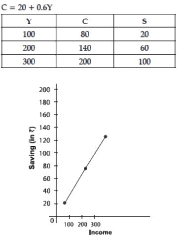
Q5: Derive a straight line saving curve using the following consumption saving on function: C = 20 + 0.6Y. Presuming the income levels to be ₹ 100, ₹ 200 and ₹ 300 crore. Calculate that level of income where consumption is equal to income.
Ans:

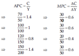
Q6: Complete the following table :

Ans:


Q7: In an economy, investment increased by 1,100 and as a result of it income increased by 5,500. Had the marginal propensity to save been 25 percent, what would have been the increase in income?
Ans: ΔY = ΔI 1/MPS
5,500 = 1100/MPS
MPS = 1100/5500 = 0.20
ΔY = 1100/0.25 = 4,400
Q8: When is an Economy in Equilibrium ? Explain with the help of saving and investment functions.
Also explain the changes that take place in an economy when the economy is not in equilibrium.
OR
Explain the determination of equilibrium level of national income using ‘saving and investment’ approach. Use diagram. Also explain the effects if savings is greater than investment.
Ans: The economy is in equilibrium at that income level at which saving = investment. The equilibrium level of income is OM as at this level S = I. When the economy is not in equilibrium, saving is not equal to investment : Suppose S > I, it means AD < AS. This leads to piling up of inventories with the producers. In order to bring down inventories to the desired level, producers cut down production which brings down AS.
The trend continues till AD = AS again and S = I where the economy is in equilibrium. Similarly, if S < I, then AD > AS. There is decrease in inventories. Producers increase production, AS rises. This continues till AD = AS.
Q9: Explain the changes that take place when Aggregate Demand and Aggregate Supply are not equal.
Answer: (i) When AD > AS, it means that the buyers are planning to buy more goods and services than the producers are planning to produce (i.e., supply).
In this situation, inventories start falling and come below the desired level, the producers expand production. This raises the income level, which keeps on rising till AD and AS are equal again.
(ii) When AD < AS, it means that the buyers are planning to buy less than what he producers are planning to produce. As a result, inventories start rising and move above the desired level. So the producers cut back on production and lay off workers. This reduces the income level i.e., AS.
This downward trend continues till AD and AS once again become equal.
Q10: In an economy planned spending is greater than planned output. Explain all the changes that will take place in the economy.
Ans: Planned spending refers to people planning to purchase final goods and services during the year. Planned output means the production units planning to produce final goods and services during the year. When planned spending is higher than planned output, the producers find the stocks falling below the desired level. They start raising production.
This raises income levels till inventories (stocks) reach the desired level and economy is in equilibrium.
Q11: (i) Define Aggregate Demand. What are its component ?
(ii) From the following data about an economy, calculate its equilibrium level of income.
(a) Marginal Propensity to Consume = 0.75
(b) Autonomous Consumption = 200
(c) Investment = 6,000
Ans: Y = C + I 1
Whereas, C = C + b(Y)
or Y = C + b(Y) + I 1
or Y = 200 + 0.75 (Y) + 6,000 1
or Y – 0.75Y = 6,200
or 0.25Y = 6,200
or Y = 6200/0.25
= 24,800or Y = ₹ 24,800
Q12: (i) Distinguish between Aggregate Demand and Aggregate Supply. (ii) From the following data about an economy calculate its equilibrium level of income.
(a) Marginal Propensity to Consume = 0.8
(b) Investment = 5,000
(c) Autonomous Consumption = 500
Ans: Y = C + I
Whereas, C = C + b(Y)
∴ Y = C + b(Y) + 500
or Y = 500 + 0.8(Y) + 5,000
or Y – 0.8Y = 5,500
or 0.2Y = 5,500
or Y = 5500/0.2
or Y = ₹ 27,500
Q13: (i) Distinguish between Autonomous Invest-ment and Induced Investment.
(ii) On the basis of the following information about an economy, calculate its equilibrium level of income.
(a) Autonomous Consumption = 100
(b) Marginal Propensity to Consume = 0.75
(c) Investment = 5,000
Ans: (i) Autonomous Investment : It is the expenditure on capital formation, which is independent of the change in income, rate of interest and rate of profit.
Induced Investment : It is the investment which is undertaken as a result of a change in the level of income or consumption. It depends upon profit expectations.
(ii) Y = C + I
and C = C + b(Y)
Here Y = C + b(Y) + I
Since S = I = 5,000
or Y = 100 + 0.75 (Y) + 5,000
or Y – 0.75 Y = 5,100
or 0.25Y = 5,100
or Y = 5100/0.25 = 5 100/25 X 100
Y = ₹ 20,400
Q14: (i) Distinguish between Autonomous Consumption and Induced Consumption.
(ii) From the following data about an economy, Calculate its equilibrium level of income.
(a) Marginal Propensity to Consume = 0.5
(b) Autonomous Consumption = 300
(c) Investment = 6,000
Ans: (i) Autonomous Consumption—The expenditure which is not influenced by income is called Autonomous Consumption. Or it refers to minimum level of consumption even when income is zero. It is indicated by C in consumption function : C = C + bY
Induced Consumption—The consumption expenditure which changes with change in income is called Induced Consumption.
(ii) Y = C + I
but C = C + b(Y) 2
∴ Y = 300 + 0.5 (Y) + 6,000 1½
or Y – 0.5 Y = 6,300
or 0.5Y = 6,300
or Y = 6300/0.5
or Y = ₹ 12,600
Q15: Explain the working of the Investment Multiplier with the help of a Numerical example.
Ans: Investment Multiplier refers to increase in national income as a multiple of a given increase in Investment. Its value is determined by MPC. The value equals :
Multiplier = 1/1-MPC or 1/MPS
Suppose increase in investment is ₹ 1000 and MPC = 0.8. The increase in National Income is in the following sequence.
(i) Increase in investment raises income of those who supply investment goods by ₹ 1000. This is the first round increase.
(ii) Since MPC = 0.8, the income earners spend ₹ 800 on consumption. This raises the income of the suppliers of consumption goods by ₹ 800. This is second round increase.
(iii) In the similar way, the third round increase in ₹ 640 = 800 × 0.8. In this way national income goes on increasing round after round.
(iv) The total increase in income is ₹ 5,000 which equals.
ΔY = ΔI × 1/1-MPC
ΔY = 1,000 × 1/1-0.08 = ₹ 5,000
Q16: What is the range of values of investment multiplier ? Clarify the relation of investment multiplier with marginal propensity to consume (MPC) and with marginal propensity to save (MPS).
Answer: Value of Investment Multiplier : (a) Minimum value of multiplier is 1 because minimum value of MPC can be zero. (b) Maximum value of multiplier may be–(infinite) because maximum value of MPC can be 1. Relationship of K (investment multiplier) with MPC and MPS (i) There is direct relationship between k and MPC. If MPC is high, k will also be high but if MPC is low, k will also be low. Thus, k varies directly with value of MPC. In short, higher the value of MPC, higher will be the value of multiplier and vice versa. (ii) There is inverse relationship between k and MPS. If MPS is high, k will be low but if MPS is low, k will be high.
Q17: Assuming that increase in investment is ₹ 1000 crore and marginal propensity to consume is 0.9, explain the working of multiplier.
Ans: Given that ΔI = 1000 and MPC = 0.9, increase in income is in the following sequence:
(i) Increase in I raises income of those who supply investment goods by ₹ 1000. This is first round increase.
(ii) Since MPC = 0.9, income earners spend ₹ 900 on consumption leading to second round increase of ₹ 900 = 1000 × 0.9
(iii) The third round increase in the similar way is ₹ 900 × 0.9 = ₹ 810.
(iv) In this way income goes on increasing round by round, with each round increase in income equal to 90 percent of the previous round.
(v) The total increase in income is :
ΔY = ΔI 1/1-MPC = 1000 X 1/1-0.6
= ₹ 10,000 crore.


