Linear Time Invariant Systems


Linear Time-Invariant systems (LTI):
Linear Time-Invariant systems (abbreviated LTI) form an important and widely used class of systems in signals and systems. In continuous time they are called Linear Time-Invariant (LTI) systems; in discrete time they are commonly referred to as Linear Shift-Invariant (LSI) systems.
Linearity and shift (time) invariance
Linearity means that if y1(t) and y2(t) are the outputs corresponding to inputs x1(t) and x2(t) respectively, then for any scalars a and b the response to ax1(t) + bx2(t) is ay1(t) + by2(t). Linearity combines the properties of additivity and homogeneity (scaling).
shift invariance (shift invariance) means that if an input x(t) produces output y(t), then the shifted input x(t - t0) produces the shifted output y(t - t0) for every real shift t0. For discrete time, replace t by n and t0 by an integer n0.
These two properties together make analysis tractable and allow the system to be completely characterised by its response to a single simple input - the unit impulse.
The unit impulse (discrete time)
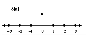
The discrete-shift unit impulse (also called the Kronecker delta) is the sequence that is zero everywhere except at one index where it equals unity. The most common choice is the origin:
δ[n] is defined by δ[0] = 1 and δ[n] = 0 for n ≠ 0.
The shifted impulse δ[n - 4] is zero for all n except at n = 4, where it equals 1. shift invariance allows us to treat shifted impulses in a straightforward way: if the system's response to δ[n] is known, the response to δ[n - k] is simply the shift of that response by k samples.
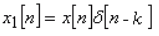
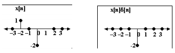
We often use impulses to "pick out" values of a sequence. In discrete time, pointwise multiplication of x[n] with δ[n - k] equals x[k]. (This property does not hold in continuous time.). This property is useful for decomposing signals and for deriving convolution expressions.
Decomposition of a discrete sequence using impulses
Any discrete sequence can be written as a weighted sum of shifted impulses. For a sequence x[n] the representation is
x[n] = Σk=-∞∞ x[k] · δ[n - k].
This identity is central to LSI theory: it shows that if we know how the system responds to each shifted impulse, we can obtain the response to any input by linear superposition and appropriate shifts.

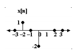
Notation and sample-sequence sketch
On paper we often represent finite sequences by listing values and indicating a start index. For example, a sequence x[n] might be shown with its first value at n = n0 and successive values to the right. The arrow notation with numbers below and above is a compact way to indicate such finite sequences and their shift origin.
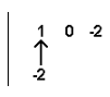
This notation is convenient for hand calculations and drawing signals on paper, though on computer text one usually writes sequences explicitly or uses the sum representation above.
The unit impulse response and system characterisation
The response of an LSI system to the unit impulse is called the impulse response and is commonly denoted by h[n] (for discrete time). For an initially relaxed linear shift-invariant system, the impulse response completely characterises the system: given h[n] we can determine the output for any input using convolution.
Example: a linear difference system
Consider the discrete-shift system defined by
y[n] = x[n] - 2x[n - 1] + 3x[n - 2].
We find the impulse response of this system by applying the unit impulse x[n] = δ[n] and computing the resulting output h[n].
Compute the impulse response as follows (each line is one logical step):
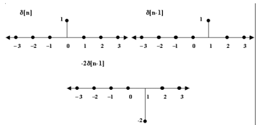
Substitute x[n] = δ[n] into the system equation.
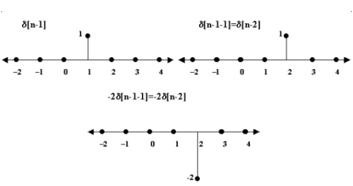
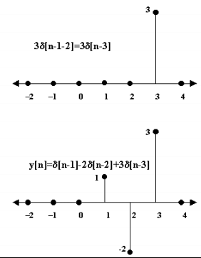
y[n] = δ[n] - 2δ[n - 1] + 3δ[n - 2]
By definition of the impulse response, h[n] = y[n] when the input is δ[n].
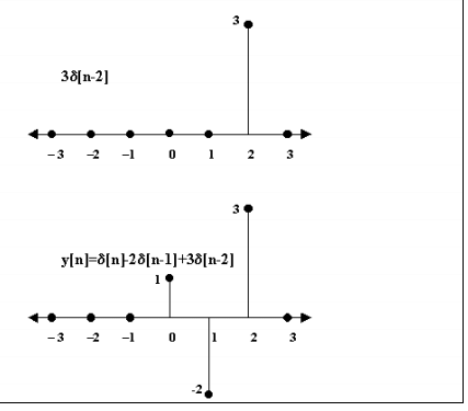
Therefore, h[n] = δ[n] - 2δ[n - 1] + 3δ[n - 2].
This describes h[n] explicitly: nonzero values occur only at n = 0, 1, 2.
Evaluate samples:
h[0] = 1
h[1] = -2
h[2] = 3
h[n] = 0 for all other n.
| n | x[n] | x[n-1] | x[n-2] | y[n] |
|---|---|---|---|---|
| ..., -1 | 0 | 0 | 0 | 0 |
| 0 | 1 | 0 | 0 | 1 |
| 1 | 0 | 1 | 0 | -2 |
| 2 | 0 | 0 | 1 | 3 |
| 3, ... | 0 | 0 | 0 | 0 |
Response to arbitrary inputs - superposition and convolution
Because the system is linear and shift invariant, the response to any arbitrary discrete input x[n] can be built from the impulse response h[n]
and the decomposition x[n] = Σ x[k] δ[n - k]. Using linearity and shift invariance we obtain the convolution sum expression for the output:
y[n] = Σk=-∞∞ x[k] · h[n - k].
Equivalently, by reindexing,
y[n] = Σm=-∞∞ h[m] · x[n - m].
This operation is called convolution of x[n] and h[n], denoted y[n] = x[n] * h[n]. For LSI systems the convolution sum is the fundamental input-output relation.
Worked example: short finite sequence
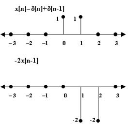
Take an input sequence with nonzero values only at n = 0 and n = 1:
x[0] = 1, x[1] = 1, and x[n] = 0 for other n.
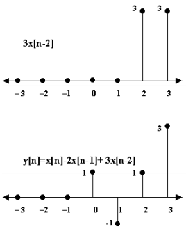
We compute the output of the example system y[n] = x[n] - 2x[n - 1] + 3x[n - 2] for this input by using decomposition and superposition.
for y[n] = x[n] - 2x[n-1] + 3x[n-2], with x[n] = δ[n] + δ[n-1]
| n | y₁[n] from δ[n] | y₂[n] from δ[n-1] | y[n] = y₁[n] + y₂[n] |
|---|---|---|---|
| ..., -1 | 0 | 0 | 0 |
| 0 | 1 | 0 | 1 |
| 1 | -2 | 1 | -1 |
| 2 | 3 | -2 | 1 |
| 3 | 0 | 3 | 3 |
| 4, ... | 0 | 0 | 0 |
x[n] = 1·δ[n] + 1·δ[n - 1].
Use linearity: the output is the sum of the outputs to each term.
The output to δ[n] is h[n] (already computed).
The output to δ[n - 1] is h[n - 1] (shifted version of h[n]).

Therefore, y[n] = h[n] + h[n - 1].
Using the sample values of h[n]: h[0] = 1, h[1] = -2, h[2] = 3, all other h[n] = 0, we can tabulate y[n] explicitly.

Adding the shifted responses sample by sample yields the final y[n]. A graphical representation or a short table shows the nonzero output values clearly.
Remarks and important consequences
- Characterisation: For any discrete LSI system, the impulse response h[n] fully characterises the system; knowledge of h[n] and convolution suffices to compute outputs for all inputs.
- Causality: An LSI system is causal if and only if h[n] = 0 for all n < 0. This means the output at time n depends only on present and past inputs.
- Stability: A discrete LSI system is BIBO (bounded-input bounded-output) stable if the impulse response is absolutely summable: Σn=-∞∞ |h[n]| < ∞. For finite-duration h[n] (FIR systems) this condition holds automatically.
- FIR and IIR: If h[n] has finite nonzero duration the system is a finite-impulse-response (FIR) system; if h[n] has infinite duration it may be an infinite-impulse-response (IIR) system.
Applications and why LSI systems matter
- Many practical signal processing and communication systems are modelled effectively as LSI systems over the interval of interest; examples include filters, digital filters used for noise removal, and many circuits approximated as linear and time-invariant.
- Convolution provides a straightforward method to compute responses, and transforms (z-transform, discrete-shift Fourier transform) convert convolution to multiplication, simplifying analysis and design.
- Impulse response measurement is a practical way to experimentally characterise an unknown LSI system: apply an impulse (or an approximation) and record the output.
Summary: For discrete-shift LSI systems the unit impulse and the impulse response are central. The impulse response h[n] yields the output for any input x[n] through the convolution sum y[n] = x[n] * h[n]. Using decomposition into weighted, shifted impulses, together with linearity and shift invariance, makes analysis systematic and straightforward.
FAQs on Linear Time Invariant Systems
| 1. What is a linear shift-invariant system? |  |
| 2. How does a linear shift-invariant system process signals? | |
| 3. What are the advantages of using linear shift-invariant systems in signal processing? | |
| 4. Can you give an example of a linear shift-invariant system? | |
| 5. How are linear shift-invariant systems relevant in real-world applications? | |


 | Explore Courses for Electrical Engineering (EE) exam |
 | Get EduRev Notes directly in your Google search |