Convective Heat Transfer: One Dimensional - 1 | Heat Transfer - Mechanical Engineering PDF Download
The rate of heat transfer in a solid body or medium can be calculated by Fourier’s law. Moreover, the Fourier law is applicable to the stagnant fluid also. However, there are hardly a few physical situations in which the heat transfer in the fluid occurs and the fluid remains stagnant. The heat transfer in a fluid causes convection (transport of fluid elements) and thus the heat transfer in a fluid mainly occurs by convection.
3.1 Principle of heat flow in fluids and concept of heat transfer coefficient
It is learnt by day-to-day experience that a hot plate of metal will cool faster when it is placed in front of a fan than exposed to air, which is stagnant. In the process, the heat is convected away, and we call the process convective heat transfer. The term convective refers to transport of heat (or mass) in a fluid medium due to the motion of the fluid. Convective heat transfer, thus, associated with the motion of the fluid. The term convection provides an intuitive concept of the heat transfer process. However, this intuitive concept must be elaborated to enable one to arrive at anything like an adequate analytical treatment of the problem.
It is well known that the velocity at which the air blows over the hot plate influences the heat transfer rate. A lot of questions come into the way to understand the process thoroughly. Like, does the air velocity influence the cooling in a linear way, i.e., if the velocity is doubled, will the heat transfer rate double. We should also suspect that the heat-transfer rate might be different if we cool the plate with some other fluid (say water) instead of air, but again how much difference would there be? These questiones may be answered with the help of some basic analysis in the later part of this module.
The physical mechanism of convective heat transfer for the problem is shown in fig.3.1.
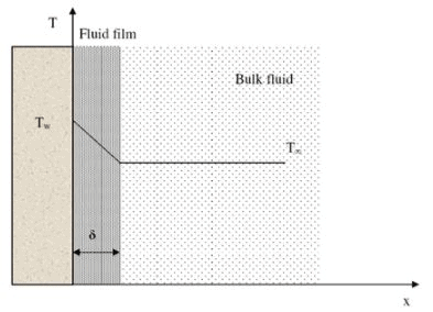
Fig. 3.1: Convective heat transfer from a heated wall to a fluid
Consider a heated wall shown in fig.3.1. The temperature of the wall and bulk fluid is denoted by  respectively. The velocity of the fluid layer at the wall will be zero. Thus the heat will be transferred through the stagnant film of the fluid by conduction only. Thus we can compute the heat transfer using Fourier’s law if the thermal conductivity of the fluid and the fluid temperature gradient at the wall is known. Why, then, if the heat flows by conduction in this layer, do we speak of convective heat transfer and need to consider the velocity of the fluid? The answer is that the temperature gradient is dependent on the rate at which the fluid carries the heat away; a high velocity produces a large temperature gradient, and so on. However, it must be remembered that the physical mechanism of heat transfer at the wall is a conduction process.
It is apparent from the above discussion that the prediction of the rates at which heat is convected away from the solid surface by an ambient fluid involves thorough understanding of the principles of heat conduction, fluid dynamics, and boundary layer theory. All the complexities involved in such an analytical approach may be lumped together in terms of a single parameter by introduction of Newton’s law of cooling,
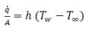 (3.1)
(3.1)
where, h is known as the heat transfer coefficient or film coefficient. It is a complex function of the fluid composition and properties, the geometry of the solid surface, and the hydrodynamics of the fluid motion.
If k is the thermal conductivity of the fluid, the rate of heat transfer can be written directly by following the Fourier’s law. Therefore, we have,
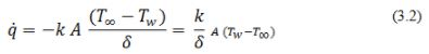
where, is the temperature gradient in the thin film where the temperature gradient is linear.
On comparing eq.3.1 and 3.2, we have,
 (3.3)
(3.3)
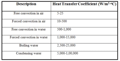
It is clear from the above expression that the heat transfer coefficient can be calculated if k and δare known. Though the k values are easily available but the δ is not easy to determine. Therefore, the above equation looks simple but not really easy for the calculation of real problems due to non-linearity of k and difficulty in determining δ. The heat transfer coefficient is important to visualize the convection heat transfer phenomenon as discussed before. In fact, δ is the thickness of a heat transfer resistance as that really exists in the fluid under the given hydrodynamic conditions. Thus, we have to assume a film of δ thickness on the surface and the heat transfer coefficient is determined by the properties of the fluid film such as density, viscosity, specific heat, thermal conductivity etc. The effects of all these parameters are lumped or clubbed together to define the film thickness. Henceforth, the heat transfer coefficient (h) can be found out with a large number of correlations developed over the time by the researchers. These correlations will be discussed in due course of time as we will proceed through the modules. Table 3.1 shows the typical values of the convective heat transfer coefficient under different situations.
Table-3.1: Typical values of h under different situations
|
57 videos|77 docs|86 tests
|
FAQs on Convective Heat Transfer: One Dimensional - 1 - Heat Transfer - Mechanical Engineering
| 1. What is convective heat transfer? |  |
| 2. How does convective heat transfer occur in one dimension? | |
| 3. What are the factors that affect convective heat transfer? | |
| 4. What are the different modes of convective heat transfer? | |
| 5. How is convective heat transfer calculated in one dimension? | |

|
4.67/5 Rating |

|
Dec 22, 2024 Last updated |

|
Explore Courses for Mechanical Engineering exam
|
|
Convective Heat Transfer: One Dimensional - 1 | Heat Transfer - Mechanical Engineering
,Exam
,Objective type Questions
,Extra Questions
,Sample Paper
,Viva Questions
,mock tests for examination
,Semester Notes
,past year papers
,shortcuts and tricks
,Summary
,ppt
,Important questions
,Convective Heat Transfer: One Dimensional - 1 | Heat Transfer - Mechanical Engineering
,Convective Heat Transfer: One Dimensional - 1 | Heat Transfer - Mechanical Engineering
,Previous Year Questions with Solutions
,Free
,video lectures
,MCQs
,study material
,practice quizzes
;


Convective Heat Transfer: One Dimensional - 1 Free PDF Download
Importance of Convective Heat Transfer: One Dimensional - 1
Convective Heat Transfer: One Dimensional - 1 Notes
Convective Heat Transfer: One Dimensional - 1 Mechanical Engineering Questions
Study Convective Heat Transfer: One Dimensional - 1 on the App
|
© EduRev
|
Education Revolution
|


|


