Procedure for Drawing Flow Nets


At every point (x, z) where there is flow, there will be a value of head h(x, z). To represent these values graphically, contours of equal head are drawn; these are called equipotential lines. A flow net is a graphical construction composed of two orthogonal families of curves: flow lines (streamlines) and equipotential lines, used to visualise two-dimensional seepage through soils and to obtain quantitative estimates of seepage quantities and pressures.
Procedure for drawing flow nets
- Establish the geometry and boundary conditions.
Draw the soil cross section to a convenient scale and mark all boundaries where head or flow is known. Indicate impermeable boundaries, free surfaces (phreatic surfaces), and any lines of known head.
- Sketch a coarse pattern of flow lines.
Begin by sketching a set of smooth, approximately spaced flow lines that satisfy the boundary conditions. Flow lines are tangent to the direction of flow at every point. Ensure that flow lines start and end on appropriate boundaries: they end on impermeable surfaces or free surfaces and pass through regions of flow between boundaries.
- Draw equipotential lines approximately orthogonal to the flow lines.
Draw curves that cut the flow lines at (approximately) right angles. Equipotential lines represent loci of constant total head. At boundaries of constant head (for example a submerged permeable face) an equipotential coincides with the boundary.
- Adjust the mesh to form curvilinear squares.
Modify the pattern so that the small regions bounded by neighbouring flow lines and equipotential lines are approximately square in the curvilinear sense. In a proper flow net each elemental cell is a curvilinear square: the head drop between successive equipotential lines is the same throughout the net and the discharge between successive flow channels is the same.
- Refine the net.
Continue adjusting and refining until the mesh is regular and the curvilinear squares are reasonably uniform in size and shape. A finer net gives better accuracy for numerical estimates.
- Count flow channels and potential drops.
Identify the number of distinct flow channels (number of spaces between adjacent flow lines cutting from upstream to downstream) and count the number of equipotential intervals (potential drops) between the upstream and downstream boundaries along a typical flow path.
Graphical rules and properties of a correct flow net
- Orthogonality: Flow lines and equipotential lines must meet at right angles everywhere.
- Curvilinear squares: The mesh elements formed by adjacent flow lines and adjacent equipotential lines should be approximately square (equal spacing in the transformed curvilinear coordinates).
- Equal head drops: The head lost between successive equipotential lines is equal throughout the net. If the total head drop between upstream and downstream is H and the net has Nd potential drops, then the head drop per interval is H/Nd.
- Equal flow between flow channels: The discharge through each flow channel is the same; if there are Nf flow channels the total discharge is the sum over these channels.
- Boundary coincidences: A permeable submerged boundary of constant head is an equipotential line. A boundary between permeable and impermeable material is a flow line. A phreatic (free) surface is a special curve that is both a flow line and an equipotential surface for atmospheric pressure at the free surface.
- Independence of direction: For a fixed set of boundary conditions the flow net is the same whether flow is considered from upstream to downstream or in the reverse direction.
Boundary conditions commonly used and their consequences
- Submerged permeable boundary (constant head): This boundary is an equipotential line because the head is the same at each point on the submerged face. Imaginary standpipes placed along the face would show the same water level.
- Permeable-impermeable interface: A boundary where permeable soil meets an impermeable stratum acts as a flow line, since no flow crosses an impermeable boundary.
- Phreatic surface (free surface): Equipotential lines intersect a phreatic surface at equal vertical intervals; the phreatic surface is a flow line subject to atmospheric pressure along it.
Quantitative use of a flow net
Once a flow net is drawn and the number of flow channels and equipotential intervals are counted, it can be used to obtain numerical estimates of seepage discharge and pore pressures. For steady, two-dimensional flow (per unit length perpendicular to the plane of the section) through a homogeneous isotropic soil, the discharge per unit width is
Q = k × H × Nf / Nd
where:
- Q = discharge per unit length perpendicular to the flow plane (m³/s per m)
- k = coefficient of permeability of the soil (m/s)
- H = total head difference between upstream and downstream boundaries (m)
- Nf = number of flow channels (number of spaces between adjacent flow lines)
- Nd = number of potential drops (number of equipotential intervals between upstream and downstream)
How to read pore pressure (head) from a flow net
- Assign the head value at the upstream equipotential as h_upstream and at the downstream equipotential as h_downstream.
- The head drop per equipotential interval is Δh = H / Nd.
- The head at the mth equipotential from upstream equals h_upstream - m Δh.
- Multiply the head at a point by the unit weight of water to obtain pore pressure (if required).
Example (illustrative calculation)
Illustrative calculation of discharge from a flow net (unit length into the page):
Given: coefficient of permeability k = 1.0 × 10⁻⁵ m/s, total head difference H = 10 m, number of flow channels Nf = 5, number of potential drops Nd = 20.
Use the discharge formula:
Q = k × H × Nf / Nd
Compute the numerical value:
Substitute the values into the formula.
Q = (1.0 × 10⁻⁵) × 10 × 5 / 20
Simplify the arithmetic.
Q = 1.0 × 10⁻⁵ × 10 × 0.25
Q = 2.5 × 10⁻⁵ m³/s per metre width.
Applications of flow nets
The graphical properties of a flow net are used in obtaining solutions for many seepage problems such as:
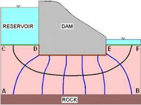
- Estimation of seepage losses from reservoirs: A flow net gives the discharge through the foundation or under a dam. The net may be constructed in the physical geometry or, for some complex shapes, in a transformed space that makes the flow easier to represent.
- Determination of uplift pressures below structures (such as gravity dams): The pressure head at any point along the base can be read from the equipotential lines and converted to uplift pressure distribution for stability checks.
- Checking the possibility of piping (boiling) at exits: At the downstream toe of an earth structure, if the upward exit hydraulic gradient approaches or exceeds a critical value, the soil may begin to boil and particles can be carried out, initiating a piping failure. Visual inspection of the flow net near the exit gives the exit gradient from the final potential drop(s).
Exit hydraulic gradient and piping
- Exit hydraulic gradient: The hydraulic gradient at the exit is the head drop across the last equipotential interval divided by the shortest vertical distance over which that head drop occurs. If the head drop per interval is Δh = H / Nd, and the distance corresponding to that interval along the flow path near the exit is l, then the approximate local gradient is Δh / l.
- Boiling or quick condition: As a simple rule, when the upward hydraulic gradient at an exit approaches unity the effective stress in a soil may reduce to zero and boiling or piping becomes possible. A more accurate estimate of the critical gradient for particle uplift is
i_c = (G_s - 1) / (1 + e)
where G_s is the specific gravity of soil solids and e is the void ratio. If the exit gradient exceeds i_c, loss of soil particles and piping are likely.
Practical checks, tips and common errors
- Always check orthogonality visually: equipotential and flow lines should intersect at roughly 90°; if not, refine the net.
- Ensure curvilinear squares are as regular as possible; large distorted cells reduce accuracy of Q = kHNf/Nd.
- In regions of rapidly varying geometry draw a denser mesh to capture the change in flow pattern.
- For layered soils or anisotropic permeability the simple flow net assumptions require modification; either use equivalent permeability approaches or more advanced analysis methods.
- Do not place image placeholders or captions inside list items; keep them in the nearest textual context as standalone blocks.
Summary
A flow net is a practical graphical tool for analysing two-dimensional steady seepage in soils. By drawing orthogonal families of flow lines and equipotential lines so that the mesh consists of curvilinear squares, one can read pore pressures, estimate seepage discharge using Q = k H Nf / Nd, and assess exit gradients for possible piping. Careful attention to boundary conditions, mesh regularity and correct counting of Nf and Nd is essential for reliable results.
FAQs on Procedure for Drawing Flow Nets
| 1. What is a flow net in civil engineering? |  |
| 2. What is the purpose of drawing a flow net? | |
| 3. How to draw a flow net in civil engineering? | |
| 4. What factors affect the flow pattern in a flow net? | |
| 5. What are the limitations of using flow nets in civil engineering? | |