General Solution To Second Order Homogeneous LTI System

General Solution to Second-Order Homogeneous LTI System
We consider the zero-input response of a standard second-order linear time-invariant (LTI) system. The homogeneous second-order differential equation in standard form is given by the following relation:

To find the general homogeneous solution, assume a trial solution of exponential form.
xh(t) = eλt
Differentiating the assumed solution with respect to time gives the first and second derivatives required to substitute into the differential equation.
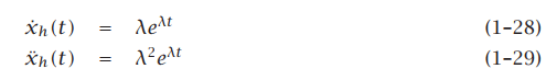
Substituting these derivatives into the homogeneous differential equation yields an algebraic equation in λ (because eλt is never zero for all t, it can be divided out).


The resulting algebraic equation is the characteristic equation. Its roots determine the behaviour of the zero-input response.
The roots of the characteristic equation, obtained from the quadratic formula, are

The nature of these roots depends on the damping ratio ζ. The sign of ζ2 - 1 leads to three distinct cases: (1) 0 ≤ ζ < 1 (underdamped), (2) ζ = 1 (critically damped), and (3) ζ > 1 (overdamped). Each case is treated below.
Case 1: 0 ≤ ζ < 1 - Underdamping
When 0 ≤ ζ < 1 the system is underdamped and ζ2 - 1 < 0, so the characteristic roots are complex conjugates.

The complex conjugate roots can be written in the form -ζωn ± jωd, where ωd is the damped natural frequency.

The general form of the real zero-input response corresponding to the complex roots is
xh(t) = e-ζωnt(c1 cos ωdt + c2 sin ωdt)
The damped natural frequency ωd is given by

To determine the constants c1 and c2, use the initial conditions x(0) = x0 and ẋ(0) = ẋ0.
Apply x(0) = x0 to the general solution.
xh(0) = x0 = c1
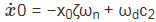
Differentiate the general solution to obtain ẋh(t).
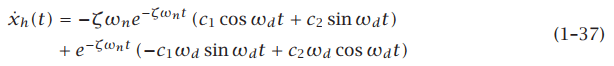
Apply the initial velocity ẋ(0) = ẋ0.

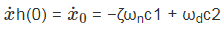
Substituting c1 = x0 into the expression for ẋ(0) gives an equation for c2.
Solving for c2 yields

Thus the zero-input response for the underdamped case can be written as

The response is an exponentially decaying sinusoid with envelope determined by e-ζωnt. A schematic illustrating typical underdamped responses for different ζ in 0 ≤ ζ < 1 is shown below.
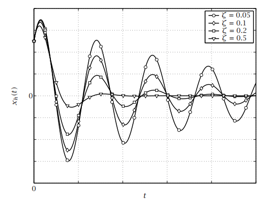
Figure 1-2 Schematic of the zero input response of an underdamped second-order linear time-invariant system.
Case 2: ζ = 1 - Critical Damping
When ζ = 1 the system is critically damped. In this case ζ2 - 1 = 0, so the two roots coincide and are real and equal.

The repeated root is
λ1 = λ2 = -ζωn = -ωn
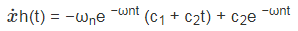
For a repeated real root, the general homogeneous solution is
xh(t) = e-ωnt(c1 + c2 t)
Use the initial conditions x(0) = x0 and ẋ(0) = ẋ0 to find c1 and c2.
Apply x(0) = x0 to the general solution.
xh(0) = x0 = c1
Differentiate xh(t) to get ẋh(t).
Apply ẋ(0) = ẋ0.

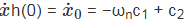
Substituting c1 = x0 into the derivative equation produces a linear equation for c2.
Solving that equation for c2 gives
Therefore the critically damped zero-input response becomes
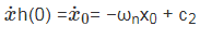
A schematic of the critically damped response is shown below.
Figure 1-3 Schematic of the zero input response of a critically damped second-order linear time-invariant system.
Case 3: ζ > 1 - Overdamping
When ζ > 1 the system is overdamped. In this case ζ2 - 1 > 0 and the characteristic equation has two distinct real roots.

Let these distinct real roots be λ1 and λ2. The general homogeneous solution is
xh(t) = c1 eλ1 t + c2 eλ2 t
Determine c1 and c2 from the initial conditions x(0) = x0 and ẋ(0) = ẋ0.
Apply x(0) = x0 to the general solution.
xh(0) = x0 = c1 + c2
Differentiate to obtain ẋh(t).
Apply the initial velocity condition ẋ(0) = ẋ0.
Solve the two linear simultaneous equations for c1 and c2.
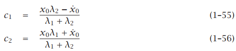
Thus the overdamped zero-input response can be expressed explicitly as

A schematic showing overdamped responses for various ζ > 1 is provided below.
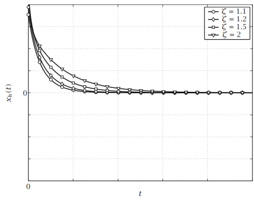
Figure 1-4 Schematic of the zero input response of an overdamped second-order linear time-invariant system.
Remarks and applications
The three canonical forms - underdamped, critically damped, and overdamped - exhaust the possible zero-input responses of a second-order homogeneous LTI system. The damping ratio ζ and natural frequency ωn are key design parameters in mechanical and aerospace applications: they determine transient settling time, overshoot, and whether oscillations occur. Typical uses include vibration analysis of single-degree-of-freedom systems, suspension design, and transient analysis of control systems.
FAQs on General Solution To Second Order Homogeneous LTI System
| 1. What is a second order homogeneous LTI system? |  |
| 2. How do you find the general solution to a second order homogeneous LTI system? | |
| 3. What is a characteristic equation of a second order homogeneous LTI system? | |
| 4. Can a second order homogeneous LTI system have complex roots in its characteristic equation? | |
| 5. Is the general solution to a second order homogeneous LTI system unique? | |