Karman Pohlhausen Approximate Method | Fluid Mechanics for Mechanical Engineering PDF Download

Karman-Pohlhausen Approximate Method For Solution Of Momentum Integral Equation Over A Flat Plate
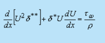
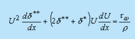
- The basic equation for this method is obtained by integrating the x direction momentum equation (boundary layer momentum equation) with respect to y from the wall (at y = 0) to a distance δX which is assumed to be outside the boundary layer. Using this notation, we can rewrite the Karman momentum integral equation as
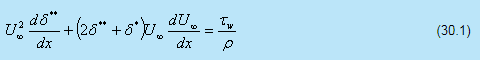
- The effect of pressure gradient is described by the second term on the left hand side. For pressure gradient surfaces in external flow or for the developing sections in internal flow, this term contributes to the pressure gradient.
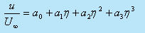
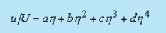
- We assume a velocity profile which is a polynomial of
 being a form of similarity variable , implies that with the growth of boundary layer as distance x varies from the leading edge, the velocity profile (u/ U∞) remains geometrically similar.
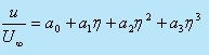
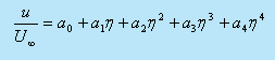
 - We choose a velocity profile in the form
 (30.2)
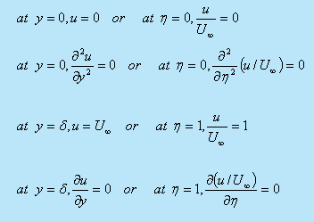
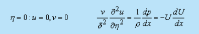
In order to determine the constants a0,a1,a2, and a3 we shall prescribe the following boundary conditions
 (30.3d)
These requirements will yield  respectively
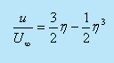
Finally, we obtain the following values for the coefficients in Eq. (30.2),  and the velocity profile becomes
- For flow over a flat plate,
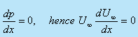 and the governing Eq. (30.1) reduces to
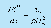 (30.5)
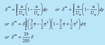
Again from Eq. (29.8), the momentum thickness is
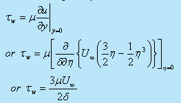
The wall shear stress is given by
substituting the values of δ** and Tw in Eq. (30.5) we get,
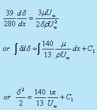
whereC1 is any arbitrary unknown constant.
- The condition at the leading edge
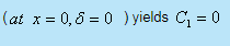
Finally we obtain,
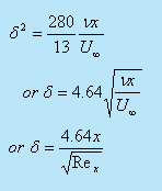 (30.8)
- This is the value of boundary layer thickness on a flat plate. Although, the method is an approximate one, the result is found to be reasonably accurate. The value is slightly lower than the exact solution of laminar flow over a flat plate . As such, the accuracy depends on the order of the velocity profile. We could have have used a fourth order polynomial instead --
In addition to the boundary conditions in Eq. (30.3), we shall require another boundary condition at
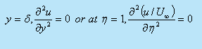
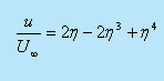
This yields the constants as 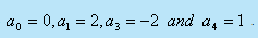 . Finally the velocity profile will be
Subsequently, for a fourth order profile the growth of boundary layer is given by
 (30.10)
Integral Method For Non-Zero Pressure Gradient Flows
- A wide variety of "integral methods" in this category have been discussed by Rosenhead . The Thwaites method is found to be a very elegant method, which is an extension of the method due to Holstein and Bohlen . We shall discuss the Holstein-Bohlen method in this section.
- This is an approximate method for solving boundary layer equations for two-dimensional generalized flow. The integrated Eq. (29.14) for laminar flow with pressure gradient can be written as
or
 (30.11)
- The velocity profile at the boundary layer is considered to be a fourth-order polynomial in terms of the dimensionless distance n = y/δ, and is expressed as
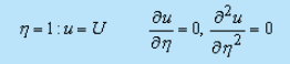
The boundary conditions are
- A dimensionless quantity, known as shape factor is introduced as
 (30.12)
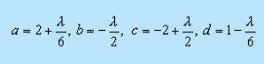
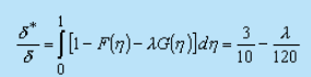
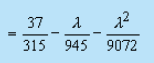
- The following relations are obtained
- Now, the velocity profile can be expressed as
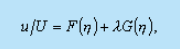 (30.13)
where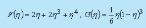
- The shear stress
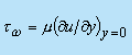 is given by
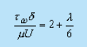 (30.14)
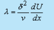
- We use the following dimensionless parameters,
 (30.15)
 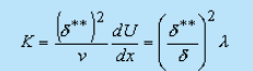 (30.16)
 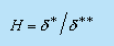 (30.17)
- The integrated momentum Eq. (30.10) reduces to
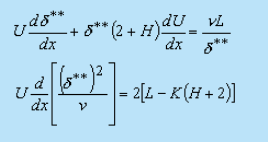 (30.18)
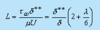
- The parameter L is related to the skin friction
- The parameter K is linked to the pressure gradient.
- If we take K as the independent variable . L and H can be shown to be the functions of K since
 (30.19)
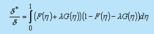
 (30.20)
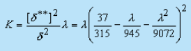 (30.21)
Therefore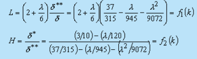
- The right-hand side of Eq. (30.18) is thus a function of K alone. Walz pointed out that this function can be approximated with a good degree of accuracy by a linear function of K so that
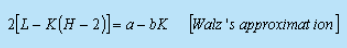
- Equation (30.18) can now be written as
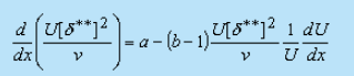
Solution of this differential equation for the dependent variable subject to the boundary condition U = 0 when x = 0 , gives
- With a = 0.47 and b = 6. the approximation is particularly close between the stagnation point and the point of maximum velocity.
- Finally the value of the dependent variable is
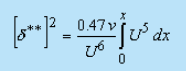 (30.22)
- By taking the limit of Eq. (30.22), according to L'Hopital's rule, it can be shown that
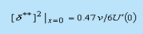
This corresponds to K = 0.0783.
- Note that
 is not equal to zero at the stagnation point. If
  is determined from Eq. (30.22),K(x) can be obtained from Eq. (30.16).
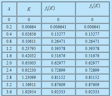
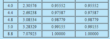
 - Table 30.1 gives the necessary parameters for obtaining results, such as velocity profile and shear stress τω The approximate method can be applied successfully to a wide range of problems.
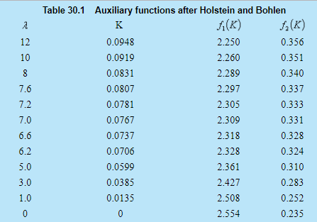
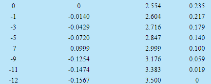
- As mentioned earlier, K and λ are related to the pressure gradient and the shape factor.
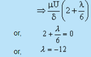
- Introduction of K and λ in the integral analysis enables extension of Karman-Pohlhausen method for solving flows over curved geometry. However, the analysis is not valid for the geometries, where λ < - 12 and λ > +12
Point of Seperation
For point of seperation, τω = 0
|
56 videos|146 docs|75 tests
|
FAQs on Karman Pohlhausen Approximate Method - Fluid Mechanics for Mechanical Engineering
| 1. What is the Karman Pohlhausen approximate method in mechanical engineering? |  |
| 2. When is the Karman Pohlhausen approximate method used in mechanical engineering? | |
| 3. How does the Karman Pohlhausen approximate method work? | |
| 4. What are the limitations of the Karman Pohlhausen approximate method? | |
| 5. Are there any alternative methods to the Karman Pohlhausen approximate method? | |


video lectures
,study material
,Karman Pohlhausen Approximate Method | Fluid Mechanics for Mechanical Engineering
,Karman Pohlhausen Approximate Method | Fluid Mechanics for Mechanical Engineering
,MCQs
,shortcuts and tricks
,Sample Paper
,Viva Questions
,Exam
,Extra Questions
,Free
,ppt
,Objective type Questions
,Karman Pohlhausen Approximate Method | Fluid Mechanics for Mechanical Engineering
,Previous Year Questions with Solutions
,Semester Notes
,Important questions
,practice quizzes
,Summary
,mock tests for examination
,past year papers
;


Karman Pohlhausen Approximate Method Free PDF Download
Importance of Karman Pohlhausen Approximate Method
Karman Pohlhausen Approximate Method Notes
Karman Pohlhausen Approximate Method Mechanical Engineering Questions
Study Karman Pohlhausen Approximate Method on the App
|
© EduRev
|
Education Revolution
|


|


