Equilibrium GDP - Macroeconomics | Macro Economics - B Com PDF Download
The Keynesian Theory
Keynes's theory of the determination of equilibrium real GDP, employment, and prices focuses on the relationship between aggregate income and expenditure. Keynes used his income‐expenditure model to argue that the economy's equilibrium level of output or real GDP may not corresPond to the natural level of real GDP. In the income‐expenditure model, the equilibrium level of real GDP is the level of real GDP that is consistent with the current level of aggregate expenditure. If the current level of aggregate expenditure is not sufficient to purchase all of the real GDP supplied, output will be cut back until the level of real GDP is equal to the level of aggregate expenditure. Hence, if the current level of aggregate expenditure is not sufficient to purchase the natural level of real GDP, then the equilibrium level of real GDP will lie somewhere below the natural level.
In this situation, the classical theorists believe that prices and wages will fall, reducing producer costs and increasing the supply of real GDP until it is again equal to the natural level of real GDP.
Sticky prices. Keynesians, however, believe that prices and wages are not so flexible. They believe that prices and wages are sticky, especially downward. The stickiness of prices and wages in the downward direction prevents the economy's resources from being fully employed and thereby prevents the economy from returning to the natural level of real GDP. Thus, the Keynesian theory is a rejection of Say's Law and the notion that the economy is self‐regulating.
Keynes's income‐expenditure model. Recall that real GDP can be decomposed into four component parts: aggregate expenditures on consumption, investment, government, and net exports. The income‐expenditure model considers the relationship between these expenditures and current real national income. Aggregate expenditures on investment, I, government, G, and net exports, NX, are typically regarded as autonomous or independent of current income. The exception is aggregate expenditures on consumption. Keynes argues that aggregate consumption expenditures are determined primarily by current real national income. He suggests that aggregate consumption expenditures can be summarized by the equation
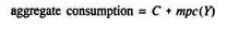
where C denotes autonomous consumption expenditure and Y is the level of current real income, which is equivalent to the value of current real GDP. The marginal propensity to consume ( mpc), which multiplies Y, is the fraction of a change in real income that is currently consumed. In most economies, the mpc is quite high, ranging anywhere from .60 to .95. Note that as the level of Y increases, so too does the level of aggregate consumption.
Total aggregate expenditure, AE, can be written as the equation
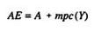
where A denotes total autonomous expenditure, or the sum C + I + G+ NX. Different levels of autonomous expenditure, A, and real national income, Y, correspond to different levels of aggregate expenditure, AE.
Equilibrium real GDP in the income‐expenditure model is found by setting current real national income, Y, equal to current aggregate expenditure, AE. Algebraically, the equilibrium condition that Y = AEimplies that
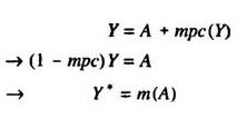
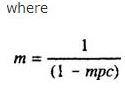
In words, the equilibrium level of real GDP, Y*, is equal to the level of autonomous expenditure, A, multiplied by m, the Keynesian multiplier. Because the mpc is the fraction of a change in real national income that is consumed, it always takes on values between 0 and 1. Consequently, the Keynesian multiplier, m, is always greater than 1, implying that equilibrium real GDP, Y*, is always a multiple of autonomous aggregate expenditure, A, which explains why m is referred to as the Keynesian multiplier.
The determination of equilibrium real national income or GDP using the income‐expenditure approach can be depicted graphically, as in Figure . This figure shows three different aggregate expenditure curves, labeled AE 1, AE 2, and A 3, which correspond to three different levels of autonomous expenditure, A 1, A 2, and A 3. The upward slope of these AE curves is due to the positive value of the mpc. As real national income Y rises, so does the level of aggregate expenditure. The Keynesian condition for the determination of equilibrium real GDP is that Y = AE. This equilibrium condition is denoted in Figure by the diagonal, 45° line, labeled Y = AE.
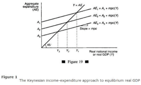
To find the level of equilibrium real national income or GDP, you simply find the intersection of the AE curve with the 45° line. The levels of real GDP that correspond to these intersection points are the equilibrium levels of real GDP, denoted in Figure as Y 1, Y 2, and Y3. Note that each AE curve corresponds to a different equilibrium level for Y. Note also that each Y is a multiple of the level of autonomous aggregate expenditure, A, as was found in the algebraic determination of the level of equilibrium real GDP.
Graphical illustration of the Keynesian theory. The Keynesian theory of the determination of equilibrium output and prices makes use of both the income‐expenditure model and the aggregate demand‐aggregate supply model, as shown in Figure .
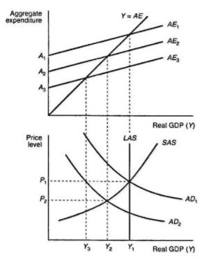
Suppose that the economy is initially at the natural level of real GDP that corresponds to Y 1 in Figure . Associated with this level of real GDP is an aggregate expenditure curve, AE 1. Now, suppose that autonomous expenditure declines, from A 1 to A 3, causing the AEcurve to shift downward from AE 1 to AE 3. This decline in autonomous expenditure is also represented by a reduction in aggregate demand from AD 1 to AD 2. At the same price level, P 1, equilibrium real GDP has fallen from Y 1 to Y 3. However, the intersection of the SAS and AD 2 curves is at the lower price level, P 2, implying that the price level falls. The fall in the price level means that the aggregate expenditure curve will not fall all the way to AE 3 but will instead fall only to AE 2. Therefore, the new level of equilibrium real GDP is at Y 2, which lies below the natural level, Y 1.
Keynes argues that prices will not fall further below P 2 because workers and other resources will resist any reduction in their wages, and this resistance will prevent suppliers from increasing their supplies. Hence, the SAS curve will not shift to the right as in the classical theory and the economy will remain at Y 2, where some of the economy's workers and resources are unemployed. Because these unemployed workers and resources earn no income, they cannot purchase goods and services. Consequently, the aggregate expenditure curve remains stuck at AE 2, preventing the economy from achieving the natural level of real GDP. Figure therefore illustrates the Keynesians' rejection of Say's Law, price level flexibility, and the notion of a self‐regulating economy.
|
59 videos|61 docs|29 tests
|
FAQs on Equilibrium GDP - Macroeconomics - Macro Economics - B Com
| 1. What is equilibrium GDP in macroeconomics? |  |
| 2. How is equilibrium GDP determined in macroeconomics? | |
| 3. What factors can cause a change in equilibrium GDP? | |
| 4. What happens if the actual GDP is above the equilibrium level? | |
| 5. How does the government intervene to achieve equilibrium GDP? | |

|
4.80/5 Rating |

|
Dec 23, 2024 Last updated |

|
Explore Courses for B Com exam
|
|
MCQs
,Objective type Questions
,Semester Notes
,ppt
,video lectures
,shortcuts and tricks
,Equilibrium GDP - Macroeconomics | Macro Economics - B Com
,practice quizzes
,Extra Questions
,Equilibrium GDP - Macroeconomics | Macro Economics - B Com
,Previous Year Questions with Solutions
,Sample Paper
,Viva Questions
,Important questions
,Summary
,mock tests for examination
,study material
,Exam
,Equilibrium GDP - Macroeconomics | Macro Economics - B Com
,Free
,past year papers
;


Equilibrium GDP - Macroeconomics Free PDF Download
Importance of Equilibrium GDP - Macroeconomics
Equilibrium GDP - Macroeconomics Notes
Equilibrium GDP - Macroeconomics B Com Questions
Study Equilibrium GDP - Macroeconomics on the App
|
© EduRev
|
Education Revolution
|


|


