The Keynesian Consumption Function (Part - 1) - Macroeconomics | Macro Economics - B Com PDF Download
Consumption Function: Concept, Keynes’s Theory and Important Features!
Introduction:
Given the aggregate supply, the level of income or employment is determined by the level of aggregate demand; the greater the aggregate demand, the greater the level of income and employment and vice versa.
Keynes was not interested in the factors determining the aggregate supply since he was concerned with the short run and the existing productive capacity. We will also not explain in detail the factors which determine the aggregate supply and will confine ourselves to explaining the determinants of aggregate demand.
Aggregate demand consists of two parts—consumption demand and investment demand. In this article we will explain the consumption demand and the factors on which it depends and how it changes over a period of time. Consumption demand depends upon the level of income and the propensity to consume. We shall explain below the meaning of the consumption function and the factors on which it depends.
The Concept of Consumption Function:
As the demand for a good depends upon its price, similarly consumption of a community depends upon the level of income. In other words, consumption is a function of income. The consumption function relates the amount of consumption to the level of income. When the income of a community rises, consumption also rises.
How much consumption rises in response to a given increase in income depends upon the marginal propensity to consume. It should be borne in mind that the consumption function is the whole schedule which describes the amounts of consumption at various levels of income.
We give below such a schedule of consumption function:
Table 6.1. Linear Consumption Function:
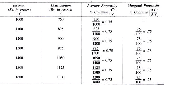
By consumption function is meant the whole schedule which shows consumption at various levels of income, whereas amount of consumption means the amount consumed at a specific level of income. The schedule described above reflects the consumption function of a community i.e., it indicates how the consumption changes in response to the change in income.
In the above schedule it will be seen that at the level of income equal to Rs. 1200 crores, the amount of consumption is Rs. 900 crores. As the national income increases to Rs. 1500 crores, the consumption rises to Rs. 1125 crores. Thus, with a given consumption function, amount of consumption is different at different levels of income.
The above schedule of consumption function reveals an important fact that when income rises, consumption also rises but not as much as the income. This fact about consumption function was emphasised by Keynes, who first of all evolved the concept of consumption function. The reason why consumption rises less than income is that a part of the increment in income is saved.
Therefore, we see that when income increases from Rs. 1000 crores to Rs. 1100 crores, the amount of consumption rises from Rs. 750 crores to 825 crores. Thus, with the increase in income by Rs. 100 crores, consumption rises by Rs. 75 crores; the remaining Rs. 25 crores are saved. Similarly, when income rises from Rs. 1100 crores to Rs. 1200 crores, the amount of consumption increases from Rs. 825 crores to Rs. 900 crores.
Here also, as a result of increase in income by Rs. 100, the amount of consumption has risen by Rs. 75 crores and the remaining Rs. 25 crores has been saved. The same applies to further increases in income and consumption. We shall see later that Keynes based his theory of multiplier on the proposition that consumption increases less than income and this theory of multiplier occupies an important place in macroeconomics.
Consumption demand depends on income and propensity to consume. Propensity to consume depends on various factors such as price level, interest rate, stock of wealth and several subjective factors. Since Keynes was concerned with short-run consumption function he assumed price level, interest rate, stock of wealth etc. constant in his theory of consumption. Thus with these factors being assumed constant in the short run, Keynesian consumption function considers consumption as a function of income. Thus
C= f(Y)
In a specific form, Keynesian function can be written as:
C = a + f(Y)
where a and b are constants. While a is intercept term of the consumption function, b stands for the slope of the consumption function and therefore represents marginal propensity to consume.
Keynesian consumption function has been depicted by CC’ curve in Fig. 6.1 in which along the X-axis national income is measured and along the Y-axis the amount of consumption is measured. In this figure, a line OZ making 45° angle with the X-axis, has been drawn. Because line OZ makes 45° angle with the X-axis every point on it is equidistant from both the X-axis and Y-axis.
Therefore, if consumption function curve coincides with 45° line OZ it would imply that the amount of consumption is equal to the income at every level of income. In this case, with the increase in income, consumption would also increase by the same amount.
As has been said above, in actual practice consumption increases less than the increase in income. Therefore, in actual practice the curve depicting the consumption function will deviate from the 45° line. If we represent the above consumption schedule by a curve, we would get the propensity to consume curve such as CC in Fig. 6.1.
It is evident from this figure that the consumption function curve CC’ deviates from the 45° line OZ. At lower levels of income, the consumption function curve CC lies above the OZ line, signifying that at these lower levels of income consumption is greater than the income.
It is so because at lower levels of income, a nation may draw upon its accumulated savings to maintain its consumption standard or it may borrow from others. As income increases, consumption also increases and at the income level OY0, consumption is equal to income.
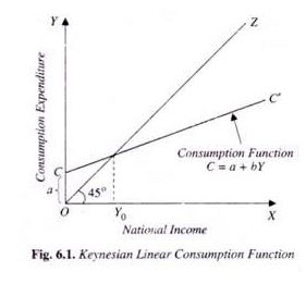
Beyond this, with the increase in income, consumption increases but less than the increase in income and therefore, consumption function curve CC lies below the 45° line OZ beyond Y0. An important point to be noted here is that beyond the level of income OY0, the gap between consumption and income is widening. The difference between consumption and income represents savings. Therefore, with the increase in income, saving gap also widens and as we shall see later, this has a significant implication in macroeconomics.
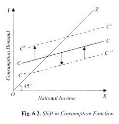
It is useful to point out here that when the consumption function of a community changes, the whole consumption function curve changes or shifts. When propensity to consume increases, it means that at various levels of income more is consumed than before.
Therefore, as a result of increase in propensity to consume of the community, the whole consumption function curve shifts upward as has been shown by the upper curve C’C’ in Fig. 6.2. On the contrary, when the propensity to consume of the community decreases, the whole consumption function curve shifts downward signifying that at various levels of income, less is consumed than before.
Average and Marginal Propensity to Consume:
There are two important concepts of propensity to consume, the one being average propensity to consume and the other marginal propensity to consume. They should be carefully distinguished, for they are equal in some cases but different in others. Consider Table 6.1, where we have calculated the average and marginal propensity to consume in columns 3 and 4. As seen above, consumption changes as income changes.
Now, how much consumption changes in response to a given change in income depends upon the average and marginal propensity to consume. Thus, propensity to consume of a community can be known by the average and marginal propensity to consume. Average propensity to consume is the ratio of the amount of consumption to total income. Therefore, average propensity to consume is calculated by dividing the amount of consumption by the total income. Thus,
APC = C/Y, where
APC stands for average propensity to consume,
C for amount of consumption, and
F for the level of income.
In the Table 6.1 it will be seen that at the level of income Rs 1000 crores, consumption expenditure is equal to Rs. 750 crores. Therefore, average propensity to consume is here equal to 750/1000 = 0.75. Likewise, when the income rises to Rs. 1200 crores, consumption rises to Rs. 900 crores.
Therefore, the average propensity to consume will be 900/1200 = 0.75. In this schedule of consumption function, the average propensity to consume is the same at all levels of income. Keynesian consumption function CC is shown in Fig. 6.3.
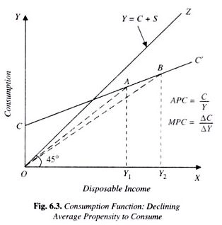
Average propensity to consume at a point on the consumption function curve can be obtained by measuring the slope of the ray from the origin to that point. For example, at income level OY1 corresponding point on the consumption function curve is A. Therefore, at OY1 income level, average propensity to consume (APC) is the slope of the ray OA.
Similarly, at income level OY2, average propensity to consume is the slope of the ray OB. It will be observed from Fig.6.3 that slope of OB is less than that of OA. Therefore, average propensity to consume at income level OY2 is less than that at income level OY1. In other words average propensity to consume has declined with the increase in disposable income.
Non-Linear Consumption Function: Average and Marginal Propensity to Consume:
In the consumption function depicted in Fig. 6.3, though average propensity to consume (C/Y) declines, marginal propensity to consume which equals ΔC/ΔY remains constant since consumption function curve CC’ is a straight line and therefore its slope (ΔC/ΔY) is constant.
But it is not necessary that marginal propensity to consume should be the same at all levels of income. We have constructed below another schedule of consumption function in which marginal propensity to consume declines with the increase in income.
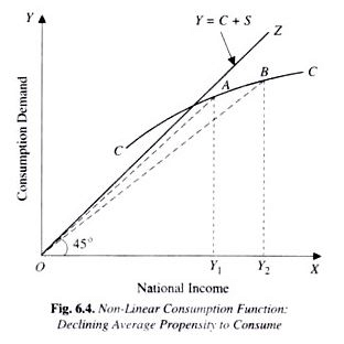
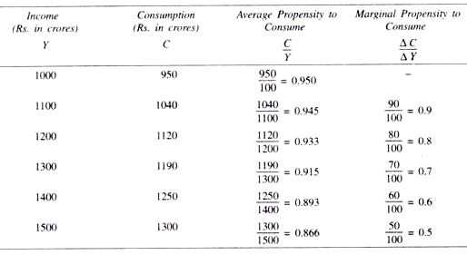
It will be seen from Table 6.2 that at the level of income of Rs. 100 crores, marginal propensity to consume is 0.9, and when income rises to Rs. 1500 crores, the marginal propensity to consume has declined to 0.5. When with the increase in income both marginal propensity to consume and average propensity to consume decline, then the curve of consumption function is not a straight line but has a shape as shown in Fig. 6.4.
From any point on the propensity to consume curve CC we can find out average propensity to consume by joining that point with the point of origin by a straight line whose slope will measure the average propensity to consume.
In Fig. 6.4, if we have to find out average propensity to consume at point A on the consumption function curve CC’, we connect point A with the origin by a straight line. Now, the slope of the line OA i.e., AY1/OY1 will indicate the average propensity to consume.
Similarly, at point B of the given consumption function CC’, the average propensity to consume will be given by the slope of the line OB which is equal to BY2/OY2. The glance at the figure will show that the slope of the line OB is smaller than the slope of the line OA. Therefore, average propensity to consume at point B or at income level OY2 is less than that at point A or income level OY1.
Table 6.2. Non-Linear Consumption Function: Average and Marginal Propensity to Consume:
Marginal Propensity to Consume:
The concept of marginal propensity to consume is very important, because from it we can know how much part of the increment in income is consumed and how much saved. Marginal propensity to consume is the ratio of change in consumption to the change in income.
Thus:
MPC = ΔC/ΔY
where, MPC stands for marginal propensity to consume,
ΔC for change in consumption, and
ΔY for change in income.
Marginal propensity to consume needs to be carefully distinguished from average propensity to consume. Whereas average propensity to consume is the ratio of total consumption to total income, i.e., C/Y, the marginal propensity to consume is the ratio of change in consumption to the change in income, i.e. ΔC/ΔY.
The concept of marginal propensity to consume can be easily understood with the aid of Table 6.2, in column 4 of which we have calculated the marginal propensity to consume at various levels of income. In this schedule when income rises from Rs. 1000 crores to Rs. 1100 crores, the consumption increases from Rs. 950 crores to Rs. 1040 crores. Here the increment in income is Rs. 100 crores and the increment in consumption is Rs. 90 crores. Therefore, marginal propensity to consume which is ΔC/ΔY is here equal to 90/100 or 0.9.
Similarly, when national income rises to Rs. 1200 crores and as a result consumption increases from Rs. 1040 crores to Rs. 1120 crores, the marginal propensity to consume is now equal to 80/100 or 0.8. In Table 6.2, it will be seen that marginal propensity to consume declines as the income rises.
It is worth noting that when with the increase in income average propensity to consume declines, marginal propensity to consume is less than average propensity to consume. This is- in accordance with the usual relationship between the average and marginal quantities. This is evident from Table 6.2.
But when average propensity to consume remains constant as in Table 6.1, marginal propensity to consume is equal to it. In Table 6.1, average propensity to consume remains constant at 0.75 and from its 4th column it will be seen that marginal propensity to consume is also 0.75.
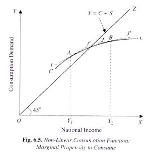
Marginal propensity to consume can be estimated by drawing the tangent at a point on the consumption function. Consider Fig. 6.5 where curve CC depicting the consumption function has been drawn. Marginal propensity to consume at point A on this will be equal to the slope of the tangent tt’ drawn at this point.
Similarly, marginal propensity to consume at point B on it is given by the slope of the tangent JJ’ drawn at this point. It will be seen that slope of the tangent JJ’ is less than the slope of the tangent tt’. Therefore, marginal propensity to consume at point B on the consumption function CC in Fig. 6.5 is smaller than the marginal propensity to consume at point A on this consumption function.
Thus, marginal propensity to consume is declining with the increases in income in the non-linear consumption function curve CC in Fig. 6.5. Thus when marginal propensity to consume declines with the increase in income, consumption function is non-linear whose slope declines as income rises. Non-linear consumption function is shown in Fig. 6.5 where the slope of the propensity to consume curve CC declines as income increases.
In Fig. 6.1 and Fig. 6.3 propensity to consume curve is a straight line i.e., the slope of the consumption function curve remains constant. Therefore, marginal propensity to consume which is given by the slope of the propensity to consume curve remains constant in Fig. 6.1.
It is worth noting that marginal propensity to consume is neither zero nor equal to one. It has been found by empirical studies that marginal propensity to consume varies between zero and unity. If the marginal propensity to consume was zero, then the whole of the increment in income would have been saved and the consumption function curve would have a horizontal shape.
As we have seen before, this is not so realistic. On the other hand, if the marginal propensity to consume was equal to unity, then the whole of the increment in income would be consumed and in that case consumption function curve would have coincided with 45° line.
Saving Function:
As mentioned above, consumption increases as income increases but less than the rise in income. We will now explain what happens to saving when income increases. Saving is defined as the part of income which is not consumed because disposable income is either consumed or saved.
Thus,
Y = C + S
S = Y – C
where Y = Disposable income, C = Consumption, S = Saving
Like consumption, saving is also a function of income. Thus, saving function can be written as
S= f(Y)
Saving function is a counterpart of a consumption function, Therefore, given a particular consumption, function, we can derive the corresponding saving function. Let us take the Keynesian consumption, namely, C = a + bY. We can derive saving function corresponding to it.
Since Y = C + S
S = Y – C
Now, substituting the above Keynesian function for C in (i) we have
S = Y – (a + bY)
= Y – a – bY
= – a + Y – bY
= – a + (1 – b) Y
Note that (1 – b) in the above saving function in (ii) is the value of marginal propensity to save where b is the value of marginal propensity to consume. Let us give a numerical example. Suppose the following consumption function is given.
C = 150 + 0.80 Y
S = Y – C
Substituting the given consumption function for C we have
S = Y – 150 – 0.80 Y
= – 150 + Y – 0.80 Y
= 150 + (1 – 0.80) Y
= – 150 + 0.20 Y
Note that 0.20 represents marginal propensity to save. It also follows from above that the sum of marginal propensity to consume and marginal propensity to save is equal to one (MPC + MPS – 1). It is important to distinguish between average propensity to save and marginal propensity to save.
Average propensity to save:
An important relationship between income and saving is described by the concept of average propensity to save. (APS). Average propensity to save is the proportion of disposable income that is saved (i.e. not consumed). Mathematically
APS = Savings/Disposable Income = S/Y
Like the average propensity to consume (APC) average propensity to save also generally varies as income increases. As seen above, average propensity to consume (APC) falls as income increases. This implies that average propensity to save will increase as income rises.
Let us derive an important relationship between average propensity to consume and average propensity to save.
Restating below the relation that income is either consumed or saved:
C + S = Y
Dividing both sides by disposable income Y we have
C/Y + S/Y + Y/Y = 1
Since C/Y is average propensity to consume and S/Y is average propensity to save, we have
APC + APS = 1
or APS = 1 – APC
This means for example, that if a society consumes 75 per cent of its disposable income, that is, APC = 0.75, then it will save 25 per cent of its disposable income or its average propensity to save (APS) will be 0.25 (1 – 0.75 = 0.25).
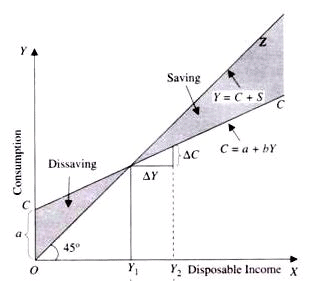
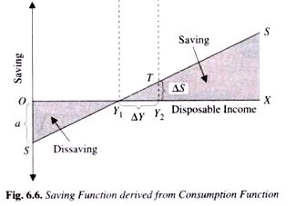
In Fig. 6.6 we have drawn the saving curve SS in the panel at the bottom. The saving curve SS shows the gap between consumption curve CC and the income curve OZ in the upper panel of Fig. 6.6. It will be seen that up to income level OY1 consumption exceeds income, that is, there is dissaving.
Beyond income level OY1, there is positive saving. It is worth mentioning that as average propensity to consume (APC) falls with the increase in income in the upper panel average propensity to save rises as income increases. Thus in Fig. 6.6 with the increase in income not only the absolute amount of saving increases, the average propensity to save also increases.
Marginal Propensity to Save (MPS):
Whereas average propensity to save indicates the proportion of income that is saved, marginal propensity to save represents how much of the additional disposable income is devoted to saving. The marginal propensity to save is therefore change in savings induced by a change in the disposable income.
Thus,
MPS = ΔS/ΔY
For example, if disposable income increases from rupees 10,000 to 12,000 and this causes planned savings to increase by Rs. 500 crores, marginal propensity to save is:
MPS = 500/2000 = 1/4 = 0.25
Since the additional income is either consumed or saved, the sum of marginal propensity to consume and marginal propensity to save is equal to one.
MPC + MPS = 1
This can be mathematically proved as under
From C + S = Y, it follows that any change in income (AF) must induce either change in consumption (AC) or change in saving (AS). Thus.
ΔC + ΔS = ΔY
Dividing both sides by ΔY we have
ΔC/ΔY + ΔS/ΔY = ΔY/ΔY = 1
MPC + MPS = 1
The concept of marginal propensity to save is graphically shown at the bottom of Fig. 6.6. It will be seen from this figure that when disposable income increases from OY1 (say Rs. 10,000) to OY2 (say Rs. 12,000), that is, ∆Y = Rs. 2000, the saving increases by Y2T, (Rs. 500), that is, ΔS is Rs. 500. Thus marginal propensity to save (MPS) is
ΔS/ΔY = Y2T/Y1Y2 = 500/2000 = 1/4 = 0.25
|
59 videos|61 docs|29 tests
|
FAQs on The Keynesian Consumption Function (Part - 1) - Macroeconomics - Macro Economics - B Com
| 1. What is the Keynesian Consumption Function? |  |
| 2. How does the Keynesian Consumption Function impact the economy? | |
| 3. What factors affect the Keynesian Consumption Function? | |
| 4. How does the marginal propensity to consume (MPC) relate to the Keynesian Consumption Function? | |
| 5. What are the limitations of the Keynesian Consumption Function? | |

|
1.7K Views |

|
4.66/5 Rating |

|
Dec 26, 2024 Last updated |

|
Explore Courses for B Com exam
|
|
Previous Year Questions with Solutions
,ppt
,mock tests for examination
,Summary
,shortcuts and tricks
,Sample Paper
,MCQs
,study material
,video lectures
,past year papers
,The Keynesian Consumption Function (Part - 1) - Macroeconomics | Macro Economics - B Com
,Extra Questions
,Viva Questions
,The Keynesian Consumption Function (Part - 1) - Macroeconomics | Macro Economics - B Com
,Semester Notes
,practice quizzes
,Objective type Questions
,Exam
,Important questions
,Free
,The Keynesian Consumption Function (Part - 1) - Macroeconomics | Macro Economics - B Com
,


The Keynesian Consumption Function (Part - 1) - Macroeconomics Free PDF Download
Importance of The Keynesian Consumption Function (Part - 1) - Macroeconomics
The Keynesian Consumption Function (Part - 1) - Macroeconomics Notes
The Keynesian Consumption Function (Part - 1) - Macroeconomics B Com Questions
Study The Keynesian Consumption Function (Part - 1) - Macroeconomics on the App
|
© EduRev
|
Education Revolution
|


|


