Saving Investment Analysis - Macroeconomics

The Saving-Investment Approach: Determination of National Income!
We have seen how equilibrium level of national income is determined by the interaction of aggregate demand and aggregate supply. The equilibrium level of national income is established at the point where aggregate demand equals aggregate supply. But there is an alternative method for the explanation of the determination of national income. This alternative method explains the determination of national income directly by intended saving and investment.
At the equilibrium level of national income OY saving and investment are equal to GE. Given the aggregate demand curve C + I, the amount of saving at income greater than OY1 exceeds investment and for income less than OY1 investment exceeds saving. It is obvious that intended saving and investment are equal only at the equilibrium level of national income and when intended saving and investment are not equal, national income will not be in equilibrium. Let us see why it is so and how national income is determined by intended saving and investment.
When at a certain level of national income, intended investment by the entrepreneurs is more than intended saving by the people, this would mean that aggregate expenditure is greater than aggregate supply of output. This will lead to the decline in inventories below the desired level. This would induce the firms to increase production, raising the level of income and employment.
The result will be that national output will be increased on account of which national income will go up. Further, when at any level of income, investment is less than saving. It means that aggregate demand is less than aggregate supply. As a result, the entrepreneurs will not be able to sell their entire output at given prices. The result will be that output will be reduced which will result in the reduction of national income.
Thus, when, at any level of national income, investment demand of the entrepreneurs is less than the intended savings of the people, the national income will decrease. It will come down to the level at which investment spending is just equal to the planned savings by the community.
But, when at any level of national income, intended investment demand on the part of the entrepreneurs is equal to intended savings of the people, it means that aggregate demand is equal to the total output or aggregate supply and therefore the national income will be equilibrium. Hence, equilibrium level of national income will be determined at the level at which the amount of intended investment by the entrepreneurs is equal to the amount of intended savings by the people. 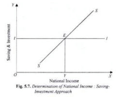
We can explain the determination of national income through saving and investment in another way. Saving represents withdrawal of some money from the income stream. On the other hand, investment represents injection of money into the income stream.
Now, if intended investment is greater than intended saving, it means that more money has been put into the income stream than has been taken out of it. As a result, income stream, i.e., flow of national income would expand.
On the contrary, if investment is less than intended saving, it means that less amount of money has been put into the income stream than has been taken out of it. The result would be that national income would decrease. But when investment is just equal to saving, it would mean that as much money has been put into the income stream as has been taken out of it. The result will be that the national income will neither increase nor decrease, i. e. it will be in equilibrium. It is thus clear that the equilibrium level of national income will be determined at the level at which the intended investment is equal to intended saving.
The determination of national income by investment and saving is illustrated in Fig. 5.7. In this figure, national income is shown along the X-axis. SS is the saving curve which shows intended saving at different levels of income, 11 curve shows investment demand i.e., intended investment.
The II investment curve has been drawn parallel to the X-axis. This is done on the assumption that in any year the entrepreneurs intend to invest a certain amount of money. This implies that we assume that investment is independent of change in income, that is, investment does not change with income.
The saving curve SS and the investment curve II intersect each other at E. That is, the intended investment and intended saving are equal at the OY level of income. Hence, OY is the equilibrium level of income. It will be seen from the Fig. 5.7 that at the level of income less than OY, the amount of intended investment is more than intended savings. As a result, income will increase.
On the contrary, at the level of income a greater than OY, the amount of intended investment is less than the intended savings with the result that income will decrease. The decrease in income will continue until it becomes equal to OY.
At the level of OY income, intended investment and intended saving are equal, so that there is neither the tendency for income to increase, nor to decrease. Hence, national income OY is determined. It is thus clear that national income is determined by the investment and saving.
Synthesis between the Two Approaches:
The determination of national income has been explained above by two methods.
The equilibrium level of national income is determined where two conditions are fulfilled:
(i) Aggregate Expenditure or Demand = Aggregate Supply of Output, and
(ii) Intended Investment = Intended Saving.
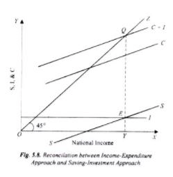
As has been explained above, the equality between aggregate demand and aggregate supply and equality between intended investment and intended saving in reality mean the same thing. This is illustrated in Fig. 5.8. It will be seen in this figure that aggregate demand curve C + I intersects aggregate supply curve OZ at point Q and thereby determines national income equal to OY. In the lower part of this diagram we have draw intended savings curve SS and intended investment curve II.
It is worthwhile to note that saving curve SS has been derived from the consumption function curve C and measures the gap between income and consumption at various levels of income.
Further, investment curve II drawn in the lower part of the figure represents the difference between consumption function curve C and aggregate demand curve C + I. This difference is the amount of intended investment assumed in this figure.
We thus see that both saving and investment curves drawn in the lower part are embedded in the upper part showing aggregate demand and aggregate supply. It is because of this that intended saving and intended investment curves also determine the same level of national income OY which is determined through the equality of aggregate demand (C + I) and aggregate supply.
Saving-Investment Approach: Algebraic Analysis:
That the level of national income is determined by the equality of planned saving and planned investment can be derived from the equilibrium condition explained above that level of income is equal to effective demand. That is,
Y = AD or AE
Where AD represents effective aggregate demand
Now in our simple economy, effective aggregate demand (AD) is equal to the sum of consumption expenditure and investment expenditure. Thus
AE or AD = C + I
or Y = C + I
Now C = Y - S
Substituting Y - S for C in equation (ii) we have
Y = Y - S + I
Y - Y + S = I
or S = I
Thus, we reach at the alternative condition of equilibrium of national income, namely, planned (intended) saving be equal to planned (intended) investment.
We can further extend saving - investment approach to show the determination of national income as a multiple of autonomous factors. Since investment is treated as autonomous of national income, its amount is taken to be a fixed amount determined exogenously. Therefore we have
I = I
Saving function as derived from the consumption function (C = a + by) can be written as
S = - a + (1 - b) Y
In equilibrium
I = - a + (1 - b) Y
(1 - b)Y = I + a
Y = 1/1-b (I + a)
where 1/1 - b is the value of multiplier and b = marginal propensity to consume and therefore 1 - b = marginal propensity to save. The equation (iv) describes the same condition which we at derived earlier. Note that a in equation (iv) is autonomous consumption which is intercept term in the consumption function.
FAQs on Saving Investment Analysis - Macroeconomics
| 1. What is saving investment analysis in macroeconomics? |  |
| 2. How is saving related to investment in macroeconomics? | |
| 3. What factors influence saving and investment levels in an economy? | |
| 4. How does saving investment analysis contribute to economic growth? | |
| 5. What are the potential risks associated with saving and investment in macroeconomics? | |