Effects of Public debt on Economic Growth (Part -2) - Public Finance | Public Finance - B Com PDF Download
Econometric Methodology:
The Model
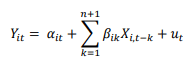
Following, a neo-classical production function framework, the functional form of the proposed Model can be written as follows,
LRY = f(LRD, LRC, LCCE) (1)
Where,
LRY = log of real GSDP,
LRD = log of real debt,
LRC = log of real credit and
LCCE = log of commercial consumption of electricity.
The Model can be written as:
LRYit —βo + βi LRDit + β2LRCit + β3LCCEit + εit (2)
Where,
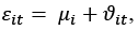
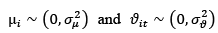 are assumed to be independent of each other and among themselves. µi and νit signify country specific fixed effects and time variants effects, respectively. The subscripts i and t denote state (i = 1 … 14) and time period considered( i= 1980/81 … … 2013/14), respectively.
The coefficients β1, β2 and β3 are the long-run elasticity estimates of gross income with respect to public debt, credit, commercial electricity consumption, respectively. The coefficient of all the explanatory variables are expected to be positive.
Any inference done on regression analysis by applying non-stationary series could lead to spurious regression. Therefore, unit-root testing and co-integration analysis are useful tools for empirical analysis. If a linear combination of two or more non-stationary series is stationary, then long-run cointegration relationship can be established among the variables. Testing for unit-roots and cointegration in panel data is helpful in establishing relationships among variables. Maddala and Wu (1999) mention that testing unit-root and cointegration in panel data increases the power of the test as compared to the respective tests done in Time series data. This paper uses four steps in its analysis: 1. Check for stationary properties of the data using panel unit root test; 2. if the series are stationary then test for the cointegration relationship, 3. in case the series are cointegrated, FMOLS and DOLS Methods are applied to measure the elasticity of income with respect to public debt, credit, and electricity consumption. 4. Causality analysis using Dumitrescu-Hurlin procedure.
Panel Unit Root Test:
Panel unit-root test can be done with two types of specification, one with a common or homogeneous unit-root process and the other with an individual or heterogeneous unit-root process. The former specification can be implemented by Levin, Li and Chu (2002) (LLC), Breitung (2000), and Hadri (1998) panel unit root tests, while the latter specification can be fulfilled by Im, Pesaran and Shin (2003) (IPS), Fisher-ADF and Fisher-PP panel unit root tests (Maddala and Wu, 1999). This paper employs four methods of panel unit root tests that are LLC, Breitung, IPS and Fisher-PP Test i.e. two tests from each categories.
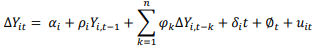
The ADF specification of LLC panel unit root test is given below.
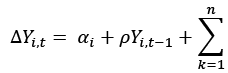
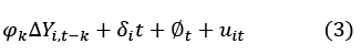
This form allows two-way fixed effects i.e. the intercept varies over state as well as time period, captured by αi and ∅t respectively. These two coefficients are basically (i − 1) state dummies and (t− 1) time dummies, respectively. The coefficient of lagged Yi is constrained to be homogeneous across all units of the panel. The null hypothesis H0 and alternative hypothesis H1 are H0: ρ= 0 and H1: ρ < 0.
In making the relevant standardization, Breitung (2000) method is different from LLC in two counts. Firstly, it removes the autoregressive portion but not the deterministic portion of the ADF equation. Secondly, the proxies for standardization are transformed and de-trended. He considers the following form to estimate the panel unit root test.
 (4)
(4)
With 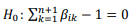 (non-stationary) and
  (stationary) for all i.
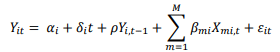
IPS (Im, Pesaran and Shin 2003) test allows heterogeneity on the coefficient of the lagged Yi variable by extending the work of LLC. The IPS procedure of testing panel unit root is based on the following model.
 (5)
(5)
With H0 : ρi =0 for all i and H1:ρi<0 for at least one i. The t-statistic, applicable for a balanced panel can be obtained by 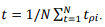 Here,tpi denotes an individual ADF t statistic to test H0 : ρi = 0 for all i.
Another alternative method of panel unit root tests applies Fisher’s (1932) results to develop tests which combine the p-values from individual unit root tests. This Method is suggested by Maddala and Wu, and by Choi.
If πi is defined as the p-value from any individual unit root test for cross-section i, then under the null of unit root for all N cross section, the asymptotic result would be,
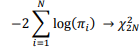 (6)
(6)
In the present paper we have reported the asymptotic X2 statistics using Phillips-Perron individual unit root tests. Choi’s result of standard normal statistics are not reported due to similarity of results. The null and alternative hypothesis for the Fisher-PP test are same as the IPS test.
The tests are done with model with intercept for all tests except the Breitung test. AIC criteria is followed to select lag length. Bandwidth is selected by taking Newey-West method using BarlettKernel spectral technique.
Panel co-integration Test:
Two varieties of co-integration test is done by following Pedroni (1999, 2004) and Kao (1999). Pedroni considers the following regression:
 (7)
(7)
In this model the X and Y are assumed to be stationary at first difference or I(1). Pedroni test is a residual based test where the residual obtained from equation (6) is tested for stationarity by estimating the following auxiliary regression:
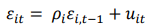 (8)
(8)
Or,
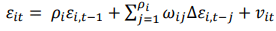 (9)
(9)
for each cross-section.
Co-integration statistics given by Pedroni is divided into two categories. The first category consists of Panel v-statistic, Panel rho-statistic, Panel PP-statistics, Panel ADF-statistics which are based on pooling along the ‘with-in’ dimension. It is done by pooling the autoregressive coefficients across the different sections of the panel for the unit-root test on the residuals. The second category is formed by Group rho-statistic, Group PP-statistic, Group ADF-statistic which are based on pooling the ‘between’ dimension. It is done by averaging the autoregressive coefficients for each member of the panel for the unit-root test of the residuals. The Kao cointegration test is also a residual based test. It distinguishes from the Pedroni test in specifying cross-section specific intercepts and homogeneous coefficients on the panel regressors.
Estimation of Panel Co-integration
Once a cointegrating relationship between the variables is established, it is useful to estimate the long-run parameters. In the presence of cointegration, OLS estimates give spurious coefficients. Therefore a number of alternative estimators are proposed such as DOLS and FMOLS among others. The major weakness of DOLS estimator is that it does not take care of the cross-sectional heterogeneity issue. Therefore, Pedroni (2000) suggested to use the FMOLS estimator that deals with the cross sectional heterogeneity, endogeneity and serial correlation problems. In small samples the FMOLS is believed to give consistent estimates. First we estimated the DOLS estimator and then to check the robustness of the results FMOLS estimator is applied.
Following, Mark and Sul (1999), the study applies a simple weighted DOLS estimator that permits for heterogeneity in the long-run variances. Similarly, feasible pooled (weighted) FMOLS estimator developed by Pedroni (2000) and Kao and Chiang (2000) is used which considers heterogeneous cointegrated panels with differences in long-run variances across cross-sections.
Dumitrescu-Hurlin causality test:
After getting long-run coefficient of three explanatory variables determining the real income, it is useful to draw information on the causal link between them which can have greater policy implications. Therefore, this study also attempts to explore on the causal link between the variables by applying Dumitrescu-Hurlin test. This test has two advantages over the Granger (1969) causality test in that in addition to the fixed coefficient accounted in Granger causality test, it considers two dimensions of heterogeneity. One for the regression model used to test Granger causality and the other is heterogeneity in the causal relationship. The detailed derivation of the Dumitrescu-Hurlin test can be found in Dumitrescu and Hurlin (2012).
Results and Implications
Panel Unit Root Test:
The empirical analysis starts with the testing of panel unit root in log-levels of real income, real public debt, real credit and electricity consumption by following four varieties of panel unit root tests viz. LLC, Breitung, IPS and Fisher-PP panel unit root test.
|
|
|
LLC |
Breitung |
IPS |
Fisher-PP |
|
|
Variable |
(t-statistics) |
(t-statistics) |
(W-Statistics) |
(Chi-square |
|
|
|||||
|
Levels |
LRY |
7.7235 |
2.9181 |
11.68 |
0.0736 |
|
|
LRD |
-2.2760** |
1.0919 |
1.7309 |
19.4651 |
|
|
LRC |
4.4096 |
1.6611 |
9.0721 |
0.4573 |
|
|
LCCE |
2.4438 |
3.6317 |
5.6921 |
20.6416 |
|
First Differences |
LRY |
-14.0529* |
-3.3658* |
-14.2520* |
344.643* |
|
|
LRD |
-6.8155* |
- 7.2473* |
-7.5748* |
137.297* |
|
|
LRC |
-6.0747* |
-5.4904* |
-5.4913* |
186.949* |
|
|
LCCE |
-16.1223* |
-5.2121* |
-17.1570* |
337.172* |
Note. 1. All tests are done on the model with an intercept except the Breitung test which is done for a model of intercept with trend. 2. Lag Lengths are set based on the AIC criterion. 3. For LLC and PPFisher test Barlet Spectral Method with Newey-West Bandwidth is applied. 4. * and ** depicts statistical significance at 1% and 5% level, respectively.
The results of panel unit root tests are reported in Table 3. It demonstrates that for the log-level series, the null of non-stationarity in variables could not be rejected for all the variables except the real debt variable. Real debt is found to be stationary in level by only the LLC test, which is refuted by other Panel Unit root tests. First difference of the log-levels variables are found to be stationary at 1 percent level of significance. Thus, the results indicate that the four variables contain a panel unit root in level.
Panel Co-integration:
As the panel unit root test results reveal that all the variables are difference stationary, we proceed to check the cointegration or long-run association of the variables by using Kao test and Pedroni Test. The model for Kao Test assumes no deterministic trend, while model for Pedroni Test assumes deterministic trend with intercept.4 Lag length is set by AIC criteria and Barlett spectral estimation procedure is applied with Newey-West automatic bandwidth. Table 4 reveals that both the Kao and Pedroni Test of cointegration suggest long-run relationship among the four variables at 1% level of significance with the exception of group-rho (between dimension) statistic in Pedroni test.
Table 4. Panel Co-integration Tests: Kao Test and Padroni Test
|
Method |
|
Statistic |
|
Kao Residual Cointegration Test |
ADF Stat. |
- 6.645* |
|
Pedroni residual cointegration test |
Panel v-Statistic |
8.151* |
|
|
Panel rho-Statistic |
-2.410* |
| Panel PP-Statistic | -6.315* | |
| Panel ADF-Statistic | -6.625* | |
| Group rho-Statistic | -0.223 | |
| Group PP-Statistic | -4.881* | |
| Group ADF-Statistic | -6.676* |
Note: 1. Trend assumption [Kao: no deterministic trend, Pedroni: Deterministic trend with intercept]; H0: No Co-integration; 2. Newey–West automatic bandwidth selection and Bartlett kernel. 2. * depicts statistical significance at 1% level.
Panel Long-run Estimates
After establishing the cointegration relationship among the variables we proceed to estimate the long-run elasticity using DOLS and check the robustness by applying FMOLS method. In the DOLS method one lead and one lag is taken. Trend specification is set with no deterministic trend and the panel option is set as Pooled (weighted) in both the methods. The long-run variance weights are derived by Barlett-kernel method with Newey-west automatic bandwidth and NW automatic lag in both the method.
Table 5 depicts the results from DOLS estimates. It reveals that public debt, institutional credit and electricity consumption are significantly affecting income. The coefficients of explanatory variables are elasticity. The coefficient for public debt in explaining income is found to be 0.33 which can be interpreted as a 1% rise in public debt will increase the income by 0.33%. The positive relationship between the public debt and economic growth could be explained by the fact that, at State level, the threshold limit of debt to GSDP is not yet been reached. The coefficient for credit and electricity variables are found to be 0.34 and 0.07 respectively. It is noticeable that the impact of public debt and institutional credit on income is similar and the impact of electricity consumption is very low. This is due to the fact that the share of electricity consumption to GSDP in each State is quite small.
Table 5. Results from DOLS Estimation (Dependent variable LRY)
|
Variable |
Coefficient |
Std. Error |
t-Statistic |
Prob. |
|
LRD |
0.3306 |
0.0346 |
9.5419 |
0.0000 |
|
LRC |
0.3390 |
0.0320 |
10.6031 |
0.0000 |
|
LCCE |
0.0729 |
0.0198 |
3.6836 |
0.0003 |
|
R-squared |
0.9893 |
|
Mean dependent var. |
11.5894 |
|
Adjusted R-squared |
0.9841 |
|
S.D. dependent var. |
0.7076 |
|
S.E. of regression |
0.0891 |
|
Sum squared resid. |
2.3111 |
| Long-run variance | 0.0129 |
Table 6 gives the estimated results obtained from FMOLS estimate. The results fairly resemble with the DOLS Method though the coefficients of various explanatory variables slightly differ. As compared to the DOLS, FMOLS assigns a slightly low coefficient to public debt variable and in turn the coefficients of the credit variable in explaining income has increased. All the explanatory variables are affecting income positively and significantly. In this case also the elasticity of income on commercial electricity consumption is low.
Table 6. Results from FMOLS Estimation (Dependent variable LRY)
|
Variable LRG LRC LCCE |
Coefficient 0.2626 0.3615 0.0734 |
Std. Error 0.0097 0.0115 0.0070 |
t-Statistic 26.9531 31.4851 10.5364 |
Prob. 0.0000 0.0000 0.0000 |
|
R-squared |
0.9805 |
Mean dependent var |
11.5950 |
|
|
Adjusted R-squared |
0.9798 |
S.D. dependent var |
0.7331 |
|
|
S.E. of regression |
0.1041 |
Sum squared resid |
4.8253 |
|
|
Long-run variance |
0.0085 |
|
|
|
Dumitrescu-Hurlin pairwise causality test:
The result of pairwise Dumitrescu-Hurlin panel causality test is reported in Table 7. The result suggests that bi-directional causality exists between public debt and economic growth which is in conformity with Puente-Ajovin and Sanso-Navarro (2015). Only, unidirectional causality is found from economic growth to credit at 10% level of significance. One way causality from economic growth to electricity consumption is also established.
Table 7. Results from Pairwise Dumitrescu-Hurlin Panel Causality Tests
|
Sample: 1980 2013 Null Hypothesis: |
Lags: 2 W-Stat. |
Zbar-Stat. |
Prob. |
|
LRD does not homogeneously cause LRY LRY does not homogeneously cause LRD |
3.9778 3.8930 |
2.9063 2.7708 |
0.0037 0.0056 |
|
LRC does not homogeneously cause LRY LRY does not homogeneously cause LRC |
2.7907 3.2070 |
1.0084 1.6739 |
0.3133 0.0941 |
|
LCCE does not homogeneously cause LRY LRY does not homogeneously cause LCCE |
2.3116 14.4135 |
0.2424 19.5908 |
0.8085 0.0000 |
|
LRC does not homogeneously cause LRD LRD does not homogeneously cause LRC |
3.4730 8.6022 |
2.0992 10.2997 |
0.0358 0.0000 |
|
LCCE does not homogeneously cause LRD LRD does not homogeneously cause LCCE |
2.4535 8.6784 |
0.4692 10.4216 |
0.6389 0.0000 |
|
LCCE does not homogeneously cause LRC LRC does not homogeneously cause LCCE |
3.5864 9.6580 |
2.2805 11.9877 |
0.0226 0.0000 |
Conclusion and Policy Implication
This study uses panel data of 14 major (non-special category) States in India during the period 1980-81 to 2013-14 to examine the influence of public debt on economic growth by controlling other relevant variables like institutional credit and commercial electricity consumption. After establishing long-run relationship among the variables, DOLS (pooled weighted) Method is applied to derive the elasticity of size of the economy (income) on public debt, credit and consumption of electricity. The study finds that economic growth is significantly and positively affected by public debt and credit. The impact of public debt and institutional credit are high and similar. The influence of electricity consumption is found to be low. To check for robustness, FMOLS (pooled weighted) estimates are also reported which give similar results. DumitrescuHurlin pairwise causality test reveals existence of bi-directional causality between public debt and economic growth. One way causality is revealed from economic growth to electricity consumption and from economic growth to credit.
The analysis reveals that at State level, expansionary debt policy will be helpful for the economy in generating higher economic growth. High economic growth will further increase the provision of institutional credit to private sector and increase the demand for energy consumption for commercial purpose. One can expand the paper by exploring on the composition of public debt and its impact on economic growth.
|
37 videos|35 docs|15 tests
|
FAQs on Effects of Public debt on Economic Growth (Part -2) - Public Finance - Public Finance - B Com
| 1. What is public debt and how does it impact economic growth? |  |
| 2. What are the potential risks of high public debt on economic growth? | |
| 3. How does public debt affect the borrowing costs of a government? | |
| 4. Can public debt ever be beneficial for economic growth? | |
| 5. How can a government manage public debt to minimize its negative impact on economic growth? | |

|
4.72/5 Rating |

|
Dec 23, 2024 Last updated |

|
Explore Courses for B Com exam
|
|
Previous Year Questions with Solutions
,Important questions
,Sample Paper
,shortcuts and tricks
,Semester Notes
,study material
,Viva Questions
,practice quizzes
,mock tests for examination
,Exam
,Objective type Questions
,Effects of Public debt on Economic Growth (Part -2) - Public Finance | Public Finance - B Com
,Extra Questions
,MCQs
,Free
,video lectures
,Summary
,Effects of Public debt on Economic Growth (Part -2) - Public Finance | Public Finance - B Com
,ppt
,Effects of Public debt on Economic Growth (Part -2) - Public Finance | Public Finance - B Com
,past year papers
;


Effects of Public debt on Economic Growth (Part -2) - Public Finance Free PDF Download
Importance of Effects of Public debt on Economic Growth (Part -2) - Public Finance
Effects of Public debt on Economic Growth (Part -2) - Public Finance Notes
Effects of Public debt on Economic Growth (Part -2) - Public Finance B Com Questions
Study Effects of Public debt on Economic Growth (Part -2) - Public Finance on the App
|
© EduRev
|
Education Revolution
|


|


