Stagflation (Part -1) - Fiscal Policy, Public Finance | Public Finance - B Com PDF Download
Meaning of Stagflation :
Economists have had known mainly two phenomena so far either of ‘inflation’ or ‘deflation’.
The former is described as a situation where too much money chases too few goods leading to a rise in prices. The later is characterized by excessive unemployment, excess capacity and fall of prices.
The decade of 1970s through 1980s has seen a new phenomenon called ‘stagflation’. It is characterized by excessive money supply and high prices on the one hand and declining productivity and unemployment on the other hand. In fact, stagflation has given rise to many problems in advanced countries like USA though developing countries are no exception to this.
The General Theory as expounded by Keynes was found to be quite inadequate to cope with a situation of stagflation particularly. Hence, doubts have been expressed whether a more General Theory than the General Theory itself as expounded by Keynes is required to cope with a situation like the above. A perusal of the performance of the American economy and its data on output, prices and unemployment show clearly that the turmoil is the rule in the American economic life.
It is true that outside- factors like wars and upheavals have been partly responsible but the fact remains that the path of the economy has been rarely smooth since 1970s through the 1980s. The data further show a new and highly disturbing element that has entered into the picture since 1960s—the economy experienced simultaneously high levels of inflation and high levels of unemployment—the condition often described by the inconvenient expression— stagflation—meaning thereby a stagnant economy with rising prices.
Throughout the 1970s, the situation worsened as both the basic factors—inflation and unemployment rates went up. The continuation of the phenomenon of stagflation is one of the unsolved and challenging problems facing contemporary macroeconomic theorists. The most vexing problem confronting economic policy makers during the last two decades has been the appearance of what is known as ‘stagflation’. The coexistence of inflation and involuntary unemployment. This type of worldwide phenomenon was not envisaged by either Classical theory or the Keynesian theory. It is a problem that deserves highest priority.
Economists all over the world, specially in USA are now focusing their attention on how to avoid stagflation rather than how to avoid either inflation or unemployment along, much of our discussion had so far been based on the simplifying assumption that there is unique full employment level of income. Below this level we have had unemployment and above it inflation. There was a no place in earlier theory or models for the two to coexist simultaneously.
Stagflation is a new phenomenon talked by certain monetary experts. It has come to be an important characteristics of an advanced monetary economy. Under it we experience, on the one hand, high prices, over full employment in certain sectors of the economy (where jobs are awaiting the right type of persons) and, on the other hand, we find symptoms of stagnation in the economy like large- scale unemployment, low agricultural and industrial production, chronic balance of payments difficulties, etc.
Thus, high prices and unemployment exist side by side in such a situation as in USA. Some economists feel that even in underdeveloped or developing countries like India symptoms of ‘stagflation’ are not difficult to discern. One of the main features of stagflation is that despite unemployment in some areas or industries, prices rise—the reason being market power of some firms and labour unions.
One great implication of stagflation is that simple monetary measures like credit curves etc. alone cannot work because the symptoms of chronic stagnation exist side by side with inflation. The decade of 1970s through 1980s is characterized in the world and in India by the phenomenon of what is called stagflation or slump-inflation; when there existed inflation with unutilized or under-utilized productive capacity along with demand recession in certain sectors of the economy.
In fact, stagflation is an international problem now—according to Randall Hinshaw economists have realized that full employment is more a range of NNP that specific point on a line. As the economy enters this range, prices begin to rise—it means that there is a tradeoff between unemployment and inflation. Accordingly, one definition of full employment is the unemployment rate at which there is an acceptable rate of inflation.
The Unemployment—Inflation Problem (Phillip’s Curve):
The idea of trade off between unemployment and inflation became a firmly established concept after the 1958 study of their relationship by A.W. Phillips, an English Economist. He published in that year a comprehensive study of unemployment and wage increases in Great Britain.
He concluded that…when the demand for labour is high and there are very few unemployed—employers bid wage rates up…each firm and each industry being continually tempted to offer a little above the prevailing rates to attract the most suitable labour from other firms and industries. As wage costs increase producers are compelled to increase their selling prices. Consequently, higher rates of inflation are generally associated with lower rates of unemployment.
Since inflation is not something we want any more of, and since the tools to curb it are at hand, why do not we just make use of them to curb it? The reason is because of a conflict of national objectives the cost of price stability in terms of the unemployment necessary to get it—is just too high! If we pursue fiscal and monetary policies to control inflation we will find ourselves with unemployment of about 8 per cent of labour force.
True, we do not want any more inflation, but we do not want any more depression either. It is clear that we cannot eat the cake and have it too! That is, both price stability and full employment at one and the same time. If we want stable prices, we have to sacrifice full employment. And if we want a high level of employment, we have to give up stable prices. In other words, we have to decide what exactly are the terms of this trade off?
Many observers have seen in this relationship the existence of an unemployment-inflation tradeoff problem. Can we simultaneously achieve high employment and price stability or must we trade off higher rates of inflation for lower levels of unemployment? The fact that price stability has not been attained in the past with low unemployment rates does not mean the existence of an unchangeable relationship. Unemployment and price level are each influenced by a great many factors. The relationship between unemployment and the price level is neither simple nor direct.
Thus, the apparent inverse relationship between unemployment and inflation, associated with growth and high employment, has been variously called the unemployment—inflation dilemma and the Phillip’s Curve. Technically speaking, the Phillip’s Curve refers to the relationship between the unemployment rate and the change in wages, a relationship in which unemployment is considered to be a major determinant of wage changes.
This unemployment-inflation relationship though has come to be called Phillip’s Curve in popular language, it would be proper to continue to refer to it as the ‘unemployment-inflation’ or the ‘U—I’ relationship. This relationship continues to be a problem of the first magnitude and every free and major industrial nation has not only recognized it but also has experimented with policies and institutions in efforts to cope with the problem.
The relation between unemployment and the rate of change of money wage rates in the UK from 1861-1957 was investigated by A.W. Phillips called Phillip’s Curve. The relation between unemployment and the rate of change of wage rates is likely to be highly non-linear.
The purpose of his study was to see whether statistical evidence supports the hypothesis that the rate of change of money wage rates in the UK can be explained by the level of unemployment and the rate of change of unemployment and if so to form some quantitative estimate of the relation between unemployment and the rate of change of money wage rates. The empirical work and the statistical evidence seems in general to support the hypothesis that the rate of change of money wage rates can be explained by the level of unemployment and the rate of change of unemployment.
Phillips has used this curve to determine that for the UK a rate of 5½ per cent unemployment is needed if wages are to be held steady, and a rate of 2½ per cent unemployment is needed if prices are to be held steady; this would mean that the wages would rise by the same percentage as productivity increases, estimated to be 2 per cent per year. Samuelson and Solow have estimated a similar curve for the United States and have found a more pessimistic figure of 5½per cent unemployment necessary for price stability, assuming that productivity increases at 2½ per cent annually.
Recent research indicates that there is an inverse relationship between the rate of inflation and the level of unemployment. It shows that in order to pursue a goal of stable prices, the economy must put up with a higher rate of unemployment; conversely, to pursue a goal of low unemployment usually a four per cent (rate considered to be full employment) the economy must be ready to suffer a higher level of inflation. Formulating a counter inflationary policy thus involves a trade-off between the goals of price stability and full employment.
When the demand for labour is high, few workers are likely to be unemployed and employer has to bid up the price at labour in order to hire them, giving rise to wage rates. Thus, wage rates rise quickly when unemployment is low. But when unemployment is high and the demand for labour is low, the workers still do not accept less wages than the prevailing wage rates. In other words, wages are sticky in the downward direction and employers are unable to get the workers accept lower wages as readily as they accept higher wages. Thus, the rate of change of money wages declines less rapidly than it rises.
The ‘Phillips Curve’ is useful because it suggests the extent to which fiscal and monetary measures can be used to reduce inflation without incurring high levels of unemployment. The value of this curve lies not in that it answers a number of questions about inflation—in fact, it raises more questions than it answers but that it makes one of the main problems in the control of inflation so vivid. There is a trade-off between wage (and price) stability and unemployment. The goals of price stability and full employment appear to be incompatible and someone must set the priority goal.
Goals in Conflict:
Implicit in the unemployment—inflation (U-I) dilemma is the proposition that full-employment and price stability, as goals, are in conflict. They are, however, not in effective conflict unless there is no desirable combination of the two that can be achieved under existing circumstances.
In the adjacent Figure 33.1, it is assumed that M1 is the maximum rate of inflation that will be tolerated by whatever constitutes the effective decision-making group.This rate is associated with zero unemployment because, presumably, higher rates of unemployment have to be compensated for by lower rates of inflation.
Similarly, Mu represents the maximum tolerable rate of unemployment and is associated with complete price stability. Mu and M1 can be connected by a curved line that reflects the maximum tolerable rate of inflation for every rate of unemployment upto Mu and vice versa. In short, all U-I points located on or within the M1, Mu curve are acceptable, each point represents a combination of an acceptable rate of inflation and an acceptable rate of unemployment. Not all the points inside the curve, however, are equally desirable.
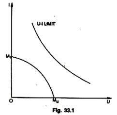
If the U-I limit curve neither touches nor intersects M1 Mu, the goals of full employment and price stability are in effective conflict. A tolerable rate of unemployment must be paid for by an unacceptable rate of inflation and the opposite also holds. If, on the other hand, the macro boundary intersects the M1 Mu curve, an acceptable rate of unemployment can be combined with an acceptable rate of inflation.
Although a trade off must still be made between a lower rate of inflation or a lower rate of unemployment, there is no effective conflict in the sense that one of the choices in the tradeoff must be unacceptable. Experience of various industrial nations suggests that high employment and price stability are in effective conflict. Nevertheless, this analysis argues that an appropriate mix of micro stabilization policies can shift the macro boundary down so that two goals are no longer in such conflicts.
Joseph A. Pechman felt that Phillips data had exaggerated the correlation between changes in wages and unemployment in UK. About Samuelson Solow thesis that the cost of price stability is an unemployment rate of 5 to 6 per cent and that a 3 per cent unemployment rate will result in 3 to 4 per cent increase in prices in the USA, he noted that this had not been established by empirical data.
There was no definite, accurate and apparent relationship that existed between changes in prices and unemployment. This, however, does not mean that the level of unemployment is not related to the price level. It simply underlines the fact that the relationship that exists is more complicated and is influenced by a large number of factors like wage rates, productivity changes, trade union activities, monetary and fiscal policies etc.
Dr. Heller remarked, “Indeed the history of our post-war period, while not conclusively proving this, seems to suggest that the 4 per cent rate of unemployment has been approximately the point at which we strike a balance between a high level of output (employment) and seasonable price stability”.
But Samuelson and Solow stated that it would now take more than 8 per cent unemployment to keep money wages from rising. It may be, perhaps, safe to conclude that price stability can be achieved, if we are satisfied with 5 to 6 per cent of labour force being unemployed. The trade-off that exists between the rate of change of prices and the unemployment is analyzed in the Fig. 33.2.
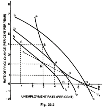
In this Figure PP is the modified Phillips Curve which expresses the relationship between the unemployment percentages and percentages of price increases. When the unemployment rate is 7 per cent, the price level will be stable at point D; but when the unemployment rate is 5 per cent prices will rise at 1 per cent per annum at point C; but when the unemployment rate falls to 4 per cent, the price will rise to 2 per cent per year at point A. Again, at 3 per cent unemployment rate, prices will rise to 4 per cent at point B.
The curves I1l1, I2I2 and I3I3 show the preferences of policy makers with respect to unemployment and inflation rates. Each of these curves is an indifference curve at which all combinations of unemployment and inflation are assumed to be equally acceptable to the authorities. For example, points S, N and R all lie on the same indifference curve I1I1and, therefore, a 4 per cent inflation and 1 per cent unemployment at point 5 or 2 per cent inflation and 3 per cent unemployment at point N and a 4 to 5 per cent unemployment with stable price level at point R are all equally acceptable to the authorities. But curves which are closer to the origin (like I1I1) are generally preferred to those which are farther away from it (like I3I3). This is because at I2I2 and I3I3 a certain level of unemployment is associated with much greater rate of increase in prices than in case of I3I3. The authorities may effect an appropriate rate of inflation with unemployment and should choose the most
economical possible combination that lies on the modified Phillips Curve PP.
This optimal combination is represented by point A on middle curve I2I2 where 4 per cent unemployment is associated with a 2 per cent inflation. If the authorities are prepared to accept more unemployment with relatively lower percentage of inflation, then, given the Phillips Curve PP, the optimum combination is determined at point C, the point of tangency between Phillips Curve and the indifference curve I’1I’1which relates higher unemployment percentage with lower percentages of inflation. At point C, the authorities will accept a 5 per cent unemployment with 1 per cent inflation. This policy of authorities determines the trade off between unemployment and inflation at a particular time.
Phillips showed that there was a stable relation during the period he studied between the unemployment rate and the rate of which the average money wage increased. Unemployment was greater when money wage rates were increasing more slowly and fell in periods when money wage rates were rising rapidly. During periods of high demand for labour, employer will tend to bid up wage rates to obtain and keep the employees they want. In periods of high unemployment, employers will not have to bid so energetically for labour, and wage rates will increase less.
But the argument was subsequently extended by others to suggest that unemployment might be reduced by allowing an inflationary rate of increase in money wage and, by extension in the average of all prices. The Phillips curve of this latter argument purports to show that there is a trade-off between inflation and unemployment, so that less of one can be obtained by accepting more of the other. It does not, however, follow either from the argument presented or from A.W. Phillips’ data that policy-makers have a menu like the one in the Fig. 33.2 from which they can simply choose their preferred combination of inflation and unemployment.
The problem is that an attempt on the part of fiscal and monetary authorities to use the curve will cause it to shift. Suppose that the unemployment rate has been 5 per cent for some time and that prices have been rising at an annual rate of 3 per cent. The government consults the Phillips curve and decides to reduce unemployment to 3 per cent by raising the inflation rate to 7 per cent. It adopts a more expansionary fiscal or monetary policy, prices and wages rise at a faster rate, and unemployment falls toward 3 per cent. The Key question now is whether unemployment can be maintained at this lower level without further accelerating the rate of inflation?
|
37 videos|35 docs|15 tests
|
FAQs on Stagflation (Part -1) - Fiscal Policy, Public Finance - Public Finance - B Com
| 1. What is stagflation and how does it relate to fiscal policy and public finance? |  |
| 2. How does fiscal policy address stagflation? | |
| 3. What are the challenges faced by public finance during stagflation? | |
| 4. Can fiscal policy alone effectively address stagflation? | |
| 5. What are some examples of fiscal policy measures used during stagflation? | |

|
4.78/5 Rating |

|
Dec 23, 2024 Last updated |

|
Explore Courses for B Com exam
|
|
study material
,Previous Year Questions with Solutions
,shortcuts and tricks
,Public Finance | Public Finance - B Com
,ppt
,MCQs
,Stagflation (Part -1) - Fiscal Policy
,Viva Questions
,Important questions
,Semester Notes
,Public Finance | Public Finance - B Com
,Free
,Sample Paper
,Stagflation (Part -1) - Fiscal Policy
,video lectures
,mock tests for examination
,past year papers
,Extra Questions
,Objective type Questions
,Exam
,practice quizzes
,Summary
,Public Finance | Public Finance - B Com
,Stagflation (Part -1) - Fiscal Policy
;


Stagflation (Part -1) - Fiscal Policy, Public Finance Free PDF Download
Importance of Stagflation (Part -1) - Fiscal Policy, Public Finance
Stagflation (Part -1) - Fiscal Policy, Public Finance Notes
Stagflation (Part -1) - Fiscal Policy, Public Finance B Com Questions
Study Stagflation (Part -1) - Fiscal Policy, Public Finance on the App
|
© EduRev
|
Education Revolution
|


|


