Transportation Problems - Elements of Operation research, Business Mathematics and Statistics | Business Mathematics and Statistics - B Com PDF Download

INTRODUCTION
Transportation problems are one of the subclasses of LPPs in which the objective is to transport various quantities of a single homogenous commodity that are initially stored at various origins, to different destinations in such a way that the transportation cost is minimum. In this unit, you will also learn about the test for optimality and degeneracy in transportation, as well as the assignment problem, the objective of which is to assign a number of origins to an equal number of destinations at minimum cost or maximum profit.
UNIT OBJECTIVES
After going through this unit, you will be able to:
-
Explain and solve transportation problems
-
Perform the optimality test using the MODI method
-
Resolve degeneracy in transportation problems
-
Describe what is unbalanced transportation
-
Solve assignment problems using the Hungarian Method
TRANSPORTATION PROBLEMS
The transportation problem is one of the subclasses of LPPs in which the objective is to transport various quantities of a single homogeneous commodity that are initially stored at various origins, to different destinations in such a way that the transportation cost is minimum. To achieve this objective we must know the amount and location of available supplies and the quantities demanded. In addition, we must know the costs that result from transporting one unit of commodity from various origins to various destinations.
Mathematical Formulation : Consider a transportation problem with m origins (rows) and n destinations (columns). Let Cij be the cost of transporting one unit of the product from the ith origin to jth destination. ai the quantity of commodity available at origin i, bj the quantity of commodity needed at destination j. xij is the quantity transported from ith origin to jth destination. This following transportation problem can be stated in the tabular form.
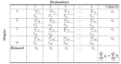
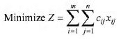
The linear programming model representing the transportation problem is given by
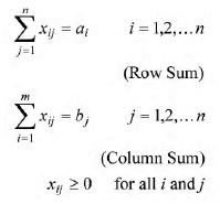
subject to the constraints
The given transportation problem is said to be balanced if
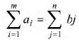
ie., if the total supply is equal to the total demand.
Definitions
Feasible Solution Any set of non-negative allocations (xij>0) which satisfies the row and column sum (rim requirement) is called a feasible solution.
Basic Feasible Solution A feasible solution is called a basic feasible solution if the number of non-negative allocations is equal to m]n[1, where m is the number of rows and n the number of columns in a transportation table.
Non-degenerate Basic Feasible Solution Any feasible solution to a transportation problem containing m origins and n destinations is said to be nondegenerate, if it contains m]n[1 occupied cells and each allocation is in independent positions.
The allocations are said to be in independent positions, if it is impossible to form a closed path.
Closed path means by allowing horizontal and vertical lines and all the corner cells are occupied.
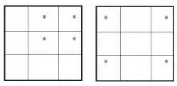
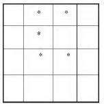
The allocations in the following tables are not in independent positions.
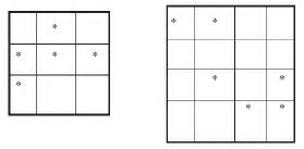
The allocations in the following tables are in independent positions.
Degenerate Basic Feasible Solution If a basic feasible solution contains less than m]n[1 non-negative allocations, it is said to be degenerate.
Optimal Solution
Optimal solution is a feasible solution (not necessarily basic) which minimizes the total cost. The solution of a transportation problem can be obtained in two stages, namely initial solution and optimum solution.
Initial solution can be obtained by using any one of the three methods, viz,
(i) North west corner rule (NWCR)
(ii) Least cost method or matrix minima method
(iii) Vogel’s approximation method (VAM)
VAM is preferred over the other two methods, since the initial basic feasible solution obtained by this method is either optimal or very close to the optimal solution.
The cells in the transportation table can be classified as occupied cells and unoccupied cells. The allocated cells in the transportation table are called occupied cells and the empty cells in a transportation table are called unoccupied cells.
The improved solution of the initial basic feasible solution is called optimal solution which is the second stage of solution, that can be obtained by MODI (modified distribution method).
North West Corner Rule
Step 1 Starting with the cell at the upper left corner (North west) of the transportation matrix we allocate as much as possible so that either the capacity of the first row is exhausted or the destination requirement of the first column is satisfied i.e., X11 = min (a1,b1).
Step 2 If b1>a1, we move down vertically to the second row and make the second allocation of magnitude x22 = min(a2 b1 – x11) in the cell (2, 1).
If b1<a1, move right horizontally to the second column and make the second allocation of magnitude X12 = min (a1, X11[b1) in the cell (1, 2).
If b1 = a1 there is a tie for the second allocation. We make the second allocations of magnitude x12 = min (a1 – a1, b) = 0 in cell (1, 2). or x21 = min (a2 – a1 – b1) = 0 in cell (2, 1).
Step 3 Repeat steps 1 and 2 moving down towards the lower right corner of the transportation table until all the rim requirements are satisfied.
Example 3.1 Obtain the initial basic feasible solution of a transportation problem whose cost and rim requirement table is the following.
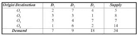
Solution Since Σai = 34 = Σbj there exists a feasible solution to the transportation problem. We obtain initial feasible solution as follows.
The first allocation is made in the cell (1, 1) the magnitude being x11 = min (5, 7) = 5. The second allocation is made in the cell (2, 1) and the magnitude of the allocation is given by x21 = min (8, 7 – 5) = 2.
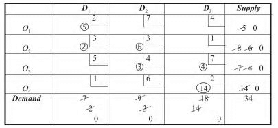
The third allocation is made in the cell (2, 2) the magnitude x22 = min (8 – 2, 9) = 6.
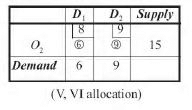
The magnitude of fourth allocation is made in the cell (3, 2) given by min (7, 9 – 6) = 3.
The fifth allocation is made in the cell (3, 3) with magnitude x33 = min (7 – 3, 14) = 4.
The final allocation is made in the cell (4, 3) with magnitude x43 = min (14, 18 – 4) = 14.
Hence, we get the initial basic feasible solution to the given T.P. and is given by X11 = 5; X21 = 2; X22 = 6; X32 = 3; X33 = 4; X43 = 14
Total cost = 2 e 5 – 3 e 2 – 3 e 6 – 3 e 4 – 4 e 7 – 2 e 14 =10 – 6 – 18 – 12 – 28 –28 = Rs 102.
Example 3.2 Determine an initial basic feasible solution to the following transportation problem using N.W.C.R
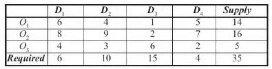
Solution The problem is a balanced TP as the total supply is equal to the total demand. Using the steps involved we find the initial basic feasible1 solution as given in the following table
The solution is given by X11 = 6; X12 = 8; X23 = 14; X33 = 1; X34 = 4
Total Cost 6 × 6 + 4 × 8 + 2 × 9 + 2 × 14 +6 × 1 + 2 × 4 = Rs 128
Least Cost or Matrix Minima Method
Step 1 Determine the smallest cost in the cost matrix of the transportation table. Let it be Cij. Allocate xij = min (ai, bj) in the cell (i, j).
Step 2 If xij = ai cross off the ith row of the transportation table and decrease bj by ai. Then go to step 3.
If xij = bj cross off the jth column of the transportation table and decrease ai by bj.
Go to step 3.
If xij = ai = bj cross off either the ith row or the jth column but not both.
Step 3 Repeat steps 1 and 2 for the resulting reduced transportation table until all the rim requirements are satisfied. Whenever the minimum cost is not unique, make an arbitrary choice among the minima.
Example 3.3 Obtain an initial feasible solution to the following TP using Matrix Minima Method.
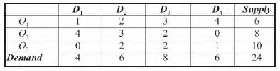
Solution Since Σai = Σbj = 24, there exists a feasible solution to the TP using the steps in the least cost method, the first allocation is made in the cell (3, 1) the magnitude being x31 = 4. This satisfies the demand at the destination D1 and we delete this column from the table as it is exhausted.
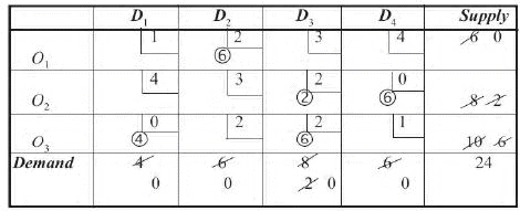
The second allocation is made in the cell (2, 4) with magnitude x24 = min (6, 8) = 6. Since it satisfies the demand at the destination D4, it is deleted from the table.
From the reduced table, the third allocation is made in the cell (3, 3) with magnitude x33 = min (8, 6) = 6. The next allocation is made in the cell (2, 3) with magnitude x23 of min (2, 2) = 2. Finally, the allocation is made in the cell (1, 2) with magnitude x12 = min (6, 6)\6. Now all the rim requirements have been satisfied and hence, the initial feasible solution is obtained.
The solution is given by x12 = 6, x23 = 2, X24 = 6, X31 = 4, X33 = 6 Since the total number of occupied cells = 5 < m + n – 1.
We get a degenerate solution.
Total cost = 6 × 2 + 2 × 2 + 6 × 0 + 4 × 0 + 6 × 2 = 12 + 4 + 12 = Rs 28.
Example 3.4 Determine an initial basic feasible solution for the following TP, using the least cost method.
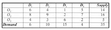
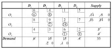
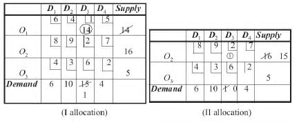
Solution Since Σai = Σ bj, there exists a basic feasible solution. Using the steps in least cost method we make the first allocation to the cell (1, 3) with magnitude X13 = min (14, 15) = 14. (as it is the cell having the least cost).
This allocation exhaust the first row supply. Hence, the first row is deleted.
From the reduced table, the next allocation is made in the next least cost cell (2, 3) which is chosen arbitrarily with magnitude X23 = Min (1, 16) = 1. This exhausts the 3rd column destination.
From the reduced table the next least cost cell is (3, 4) for which allocation is made with magnitude min (4, 5) = 4. This exhausts the destination D4 requirement.
Delete this fourth column from the table. The next allocation is made in the cell (3, 2) with magnitude X32 = Min (1, 10) = 1. This exhausts the 3rd origin capacity.
Hence, the 3rd row is exhausted. From the reduced table the next allocation is given to the cell (2,1) with magnitude X21 = min (6, 15) = 6. This exhausts the first column requirement. Hence, it is deleted from the table.
Finally, the allocation is made to the cell (2, 2) with magnitude X22 = Min (9, 9) = 9 which satisfies the rim requirement. These allocation are shown in the transportation table as follows.
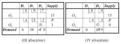
The following table gives the initial basic feasible solution.
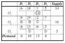
The solution is given by X13=14; X21=6; X22= 9; X23= 1; X32= 1; X34= 4
Transportation cost = 14 ×1 × 6 × 8 + 9 × 9 + 1 × 2 + 3 × 1 + 4 × 2
= Rs 156.
|
124 videos|176 docs
|
FAQs on Transportation Problems - Elements of Operation research, Business Mathematics and Statistics - Business Mathematics and Statistics - B Com
| 1. What is a transportation problem in the context of operations research, business mathematics, and statistics? |  |
| 2. How can linear programming be used to solve transportation problems? | |
| 3. What are the key elements involved in solving a transportation problem? | |
| 4. What are the different methods to solve transportation problems? | |
| 5. Can transportation problems have multiple optimal solutions? | |


Important questions
,Sample Paper
,study material
,Semester Notes
,Extra Questions
,shortcuts and tricks
,ppt
,Transportation Problems - Elements of Operation research
,video lectures
,Transportation Problems - Elements of Operation research
,Free
,Summary
,Business Mathematics and Statistics | Business Mathematics and Statistics - B Com
,Business Mathematics and Statistics | Business Mathematics and Statistics - B Com
,Objective type Questions
,Previous Year Questions with Solutions
,Business Mathematics and Statistics | Business Mathematics and Statistics - B Com
,practice quizzes
,Viva Questions
,past year papers
,Exam
,Transportation Problems - Elements of Operation research
,MCQs
,mock tests for examination
;


Transportation Problems - Elements of Operation research, Business Mathematics and Statistics Free PDF Download
Importance of Transportation Problems - Elements of Operation research, Business Mathematics and Statistics
Transportation Problems - Elements of Operation research, Business Mathematics and Statistics Notes
Transportation Problems - Elements of Operation research, Business Mathematics and Statistics B Com Questions
Study Transportation Problems - Elements of Operation research, Business Mathematics and Statistics on the App
|
© EduRev
|
Education Revolution
|


|


within 7 days!