Linear Ordinary Differential Equations of First and Second Order - 1 | Physics for IIT JAM, UGC - NET, CSIR NET PDF Download

First-order differential equations involve the first derivative of an unknown function y (t). They are of the form:
y′ = f(t, y),
where y′ = dy/dt, and f (t, y) is a given function. These notes cover two main types: linear and separable equations, with a focus on solution methods and exam-relevant techniques.
Linear First-Order Differential Equations
A linear first-order differential equation has the form:
y′ + p(t)y = g(t),
where p (t) and g (t) are functions of t. The solution method is the integrating factor technique.
Method of Integrating Factors
Multiply both sides of the equation by an integrating factor μ (t): μ(t)y′ + μ(t)p(t)y = μ(t)g(t).
Choose μ (t) such that the left-hand side is the derivative of a product: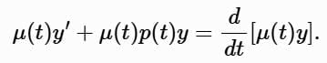 By the product rule, d/dt [μ (t) y] = μ (t) y ′ + μ ′ (t) y . Equate coefficients of y:
μ′(t)y = μ(t)p(t)y ⟹ μ′(t) = μ(t)p(t).
This simplifies to: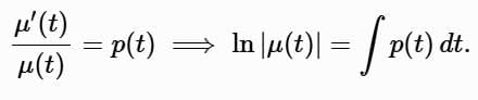 Thus, the integrating factor is:
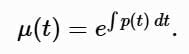 The constant of integration can be omitted, as any μ (t) of this form works. The equation becomes:
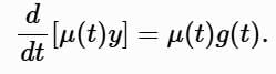
Integrate both sides: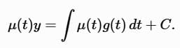
Solve for y: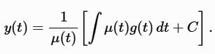
Examples
Example 1: Solve y ′ + ay = b , where a ≠ 0 , with no initial condition
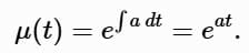
Here, p (t) = a , g (t) = b. The integrating factor is:
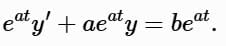
Multiply through:
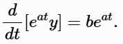
The left-hand side is:
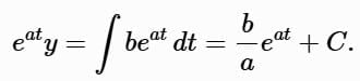
Integrate:
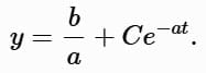
Solve for y :
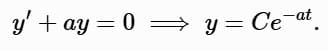
For the homogeneous case (b = 0 ):
The general solution combines the homogeneous and particular solutions, confirming the result.
Example 2: Solve y ′ + y = e2t
Here, p (t) = 1 , g (t) = e2t . The integrating factor is:
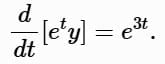
Multiply through:
The left-hand side is:
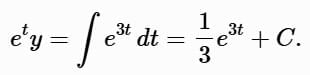
Integrate:
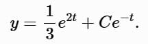
Solve for y:
Verify by substituting back to ensure correctness (a good exam practice).
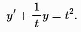
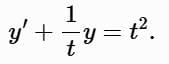
Example 3: Solve ty ′ + y = t3, y ( − 1 ) = 3
Rewrite in standard form (t ≠ 0):
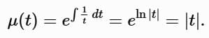
Here, p(t) = 1/t, g (t) = t2. The integrating factor is:
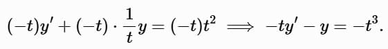
Since y (− 1) = 3 implies t < 0 , use μ (t) = − t for t < 0 . Multiply through:
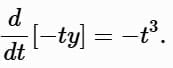
The left-hand side is:
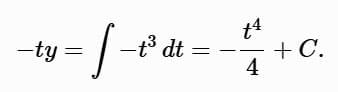
Integrate:
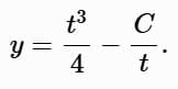
Solve for y:
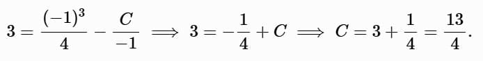
Apply the initial condition y (− 1) = 3:
Thus:
The solution is valid for t < 0 , as t = 0 makes the denominator undefined.
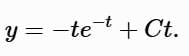
Example 4: Solve t y ′ − y = t2e − t, t > 0
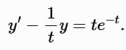
Rewrite in standard form:
Here, p(t) = -1/t, g (t) = te−t. The integrating factor is:
Multiply through:
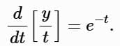
The left-hand side is:
Integrate:
Solve for y :
No initial condition is provided, so this is the general solution for t > 0.
Separable Equations
A separable equation is of the form: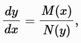
where M (x) and N (y) depend only on x and y , respectively.
Rewrite as: N(y)dy = M(x)dx.
Integrate both sides to find the solution, often implicitly:
Examples
Example 1: Solve y ′ = − 2x/y, y (π) = 2
Rewrite: y dy = −2x dx.
Integrate:Apply the initial condition y (π) = 2:
4 = −2π2 + K ⟹ K = 4 + 2π2.
Thus,
y2 = −2x2 + 4 + 2π2.
Solve explicitly:Since y (π) = 2, take the positive root. The solution is valid where − 2x2 + 4 + 2π2 > 0.

Example 2: Solve y ′ = 3x2(1 + y2) , y (0) = 0
Rewrite:
Integrate:
Apply the initial condition y (0) = 0:
arctan 0 = 0 + C ⟹ C = 0.
Thus:
arctan y = x3 ⟹ y = tan(x3).
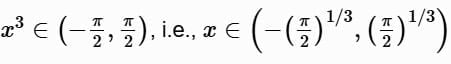
The solution is defined where
Example 3: Solve 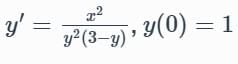
Rewrite: y2(3 − y)dy = x2dx.
Integrate: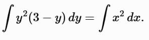 Left-hand side:
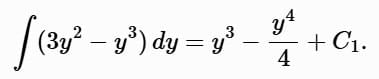 Right-hand side:
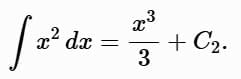
Thus: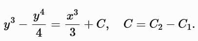
Apply the initial condition y (0) = 1: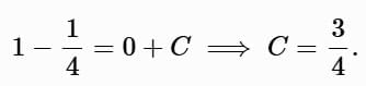 Thus:
Thus: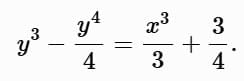 To find the valid interval, note that y ′ is undefined at y = 0 or y = 3 . Check for x values:
At y = 0: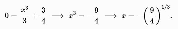
At y = 3:
Since y (0) = 1 , the solution is valid between these points: − (9/4)1/3 < x < 181/3.
Existence and Uniqueness
For a linear equation y ′ + p (t) y = g (t), y (t0) = y0:
- If p (t) and g (t) are continuous on an open interval containing t0, the solution exists and is unique on that interval.
For a nonlinear equation y′ = f(t, y), y (t0) = y0:
- If f and ∂f/∂y are continuous in a rectangle around (t0, y0), a unique solution exists in some interval around t0.
Examples
Example 1: Largest interval for ty′ + y = t3, y (− 1) = 3
Standard form:
Here, p (t) = 1/t , g (t) = t2, undefined at t = 0 . Since t0 = − 1 , the solution is valid for t < 0.
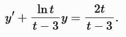
Example 2: Largest interval for (t − 3) y ′+ (ln t) y = 2 t , y (1) = 2
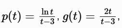
Standard form:
Here,
undefined at t = 0 (due to ln t ) and t = 3. Since t0 = 1 , the interval is 0 < t < 3.
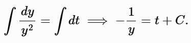
Example 3: Blow-up for y ′ = y2, y ( 0 ) = 1
Separate variables:
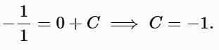
Apply y(0) = 1:
Thus:
The solution blows up at t = 1 , undefined beyond this point.
FAQs on Linear Ordinary Differential Equations of First and Second Order - 1 - Physics for IIT JAM, UGC - NET, CSIR NET
| 1. What is a linear ordinary differential equation of first order? |  |
| 2. How do you solve a linear ordinary differential equation of first order? | |
| 3. What is a linear ordinary differential equation of second order? | |
| 4. Can linear ordinary differential equations of second order have non-constant coefficients? | |
| 5. What are the applications of linear ordinary differential equations in physics? | |


CSIR NET
,Previous Year Questions with Solutions
,Viva Questions
,UGC - NET
,Important questions
,Free
,CSIR NET
,practice quizzes
,study material
,Semester Notes
,mock tests for examination
,shortcuts and tricks
,Summary
,Extra Questions
,CSIR NET
,Exam
,MCQs
,ppt
,video lectures
,past year papers
,Objective type Questions
,Linear Ordinary Differential Equations of First and Second Order - 1 | Physics for IIT JAM
,Linear Ordinary Differential Equations of First and Second Order - 1 | Physics for IIT JAM
,Linear Ordinary Differential Equations of First and Second Order - 1 | Physics for IIT JAM
,UGC - NET
,Sample Paper
,UGC - NET
;


Linear Ordinary Differential Equations of First and Second Order - 1 Free PDF Download
Importance of Linear Ordinary Differential Equations of First and Second Order - 1
Linear Ordinary Differential Equations of First and Second Order - 1 Notes
Linear Ordinary Differential Equations of First and Second Order - 1 Physics Questions
Study Linear Ordinary Differential Equations of First and Second Order - 1 on the App
|
© EduRev
|
Education Revolution
|


|


within 7 days!