Linear Ordinary Differential Equations of First and Second Order - 2 | Physics for IIT JAM, UGC - NET, CSIR NET PDF Download
Modeling with first order equations
General modeling concept: derivatives describe “rates of change”.
Model I: Exponential growth/decay.
Q(t) = amount of quantity at time t Assume the rate of change of Q(t) is proportional to the quantity at time t. We can write
 r : rate of growth/decay
If r > 0: exponential growth
If r < 0: exponential decay
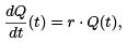
Differential equation:
Q′ = rQ, Q(0) = Q0 .
Solve it: separable equation.
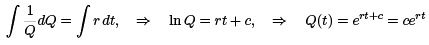
Here r is called the growth rate. By IC, we get Q(0) = C = Q0. The solution is
Q(t) = Q0ert .
Two concepts:
- For r > 0, we define Doubling time TD , as the time such that Q(TD ) = 2Q0 .

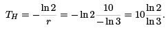
- For r < 0, we define Half life (or half time) TH , as the time such that


Note here that TH > 0 since r < 0.
NB! TD , TH do not depend on Q0 . They only depend on r.
Example 1. If interest rate is 8%, compounded continuously, find doubling time.
Answer.Since r = 0.08, we have TD = 
Example 2. A radio active material is reduced to 1/3 after 10 years. Find its half life.
Answer.
Model:  = rQ, r is rate which is unknown. We have the solution Q(t) = Q0ert .
So
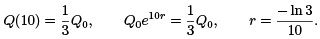
To find the half life, we only need the rate r
Model II: Interest rate/mortgage problems.
Example 3. Start an IRA account at age 25. Suppose deposit $2000 at the beginning and $2000 each year after. Interest rate 8% annually, but assume compounded continuously.
Find total amount after 40 years.
Answer. Set up the model: Let S (t) be the amount of money after t years
 = 0.08S + 2000, S (0) = 2000.
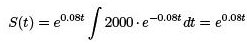
This is a first order linear equation. Solve it by integrating factor
S ′ − 0.08S = 2000, µ = e−0.08t
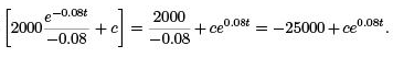
By IC, S (0) = −25000 + c = 2000, C = 27000,
we get
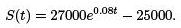
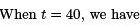
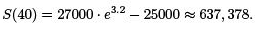
Compare this to the total amount invested: 2000 + 2000 ∗ 40 = 82, 000.
Example 4: A home-buyer can pay $800 per month on mortgage payment. Interest rate is r annually, (but compounded continuously), mortgage term is 20 years. Determine maximum amount this buyer can afford to borrow. Calculate this amount for r = 5% and r = 9% and observe the difference.
Answer. Set up the model: Let Q(t) be the amount borrowed (principle) after t years
 = rQ(t) − 800 ∗ 12
The terminal condition is given Q(20) = 0. We must find Q(0).
Solve the differential equation:
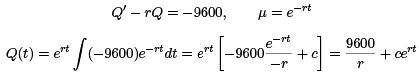 .
.
By terminal condition
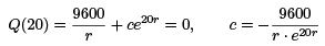
so we get

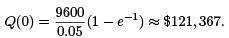
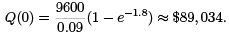
Now we can get the initial amount
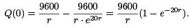
If r = 5%, then
If r = 9%, then
We observe that with higher interest rate, one could borrow less.
Model III: Mixing Problem.
Example 5. At t = 0, a tank contains Q0 lb of salt dissolved in 100 gal of water. Assume that water containing 1/4 lb of salt per gal is entering the tank at a rate of r gal/min. At the same time, the well-mixed mixture is draining from the tank at the same rate. (1). Find the amount of salt in the tank at any time t ≥ 0. (2). When t → ∞, meaning after a long time, what is the limit amount QL?
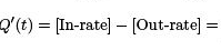
Answer. Set up the model: Q(t) = amount (lb) of salt in the tank at time t (min) Then, Q′(t) = [in-rate] − [out-rate].
In-rate: r gal/min × 1/4 lb/gal = r/4 lb/min
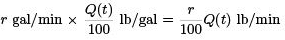
concentration of salt in the tank at time t = 
Out-rate:
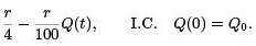
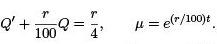
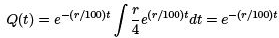
(1). Solve the equation
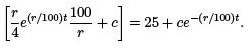
By IC
Q(0) = 25 + c = Q0, c = Q0 − 25,
we get
Q(t) = 25 + (Q0 − 25)e−(r/100)t .
(2). As t → ∞, the exponential term goes to 0, and we have
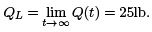
We can also observed intuitively that, as time goes on for long, the concentration of salt in the tank must approach the concentration of the salt in the inflow mixture, which is 1/4. Then, the amount of salt in the tank would be 1/4 × 100 = 25 lb, as t → +∞.
Example 6. Tank contains 50 lb of salt dissolved in 100 gal of water. Tank capacity is 400 gal. From t = 0, 1/4 lb of salt/gal is entering at a rate of 4 gal/min, and the well-mixed mixture is drained at 2 gal/min. Find:
(1) time t when it overflows;
(2) amount of salt before overflow;
(3) the concentration of salt at overflow.
Answer.(1). Since the inflow rate 4 gal/min is larger than the outflow rate 2 gal/min, the tank will be filled up at tf :
 = 150min.
(2). Let Q(t) be the amount of salt at t min.
In-rate: 1/4 lb/gal × 4 gal/min = 1 lb/min
Out-rate: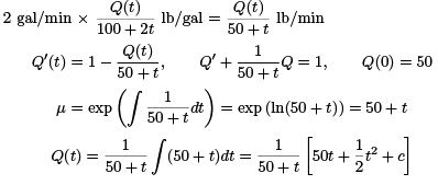
By IC
Q(0) = c/50 = 50, c = 2500,
We get
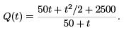
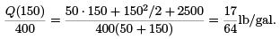
(3). The concentration of salt at overflow time t = 150 is
Model IV: Air resistance
Example 7. A ball with mass 0.5 kg is thrown upward with initial velocity 10 m/sec from the roof of a building 30 meter high. Assume air resistance is |v|/20. Find the max height above ground the ball reaches.
Answer. Let S (t) be the position (m) of the ball at time t sec. Then, the velocity is v(t) = dS/dt, and the acceleration is a = dv/dt. Let upward be the positive direction. We have by Newton’s Law:
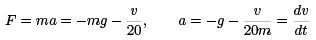
Here g = 9.8 is the gravity, and m = 0.5 is the mass. We have an equation for v:
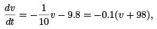
so
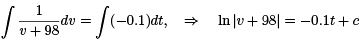
which gives

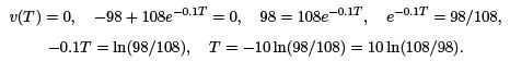
By IC:

To find the position S , we use S ′ = v and integrate

By IC for S ,
S (0) = −1080 + c = 30, c = 1110, S (t) = −98t − 1080e−0.1t + 1110.
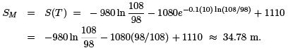
At the maximum height, we have v = 0. Let’s find out the time T when max height is reached.
So the max height SM is
Other possible questions:
- Find the time when the ball hit the ground.
Solution: Find the time t = tH for S(tH ) = 0.
- Find the speed when the ball hit the ground.
Solution: Compute |v(tH )|.
- Find the total distance traveled by the ball when it hits the ground.
Solution: Add up twice the max height SM with the height of the building.
Autonomous equations and population dynamics
Definition: An autonomous equation is of the form y′ = f (y), where the function f for the derivative depends only on y, not on t.
Simplest example: y′ = ry, exponential growth/decay, where solution is y = y0ert .
Definition: Zeros of f where f (y) = 0 are called critical points or equilibrium points, or equilibrium solutions.
Why? Because if f (y0) = 0, then y(t) = y0 is a constant solution. It is called an equilibrium.
Question: Is an equilibrium stable or unstable?
Example 1. y′ = y(y − 2). We have two critical points: y1 = 0, y2 = 2.
We see that y1 = 0 is stable, and y2 = 2 is unstable.
Example 2. For the equation y′ = f (y) where f (y) is given in the following plot:
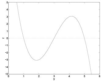
(A). What are the critical points?
(B). Are they stable or unstable?
(C). Sketch the solutions in the t − y plan, and describe the behavior of y as t → ∞ (as it depends on the initial value y(0).)
Answer.(A). There are three critical points: y1 = 1, y2 = 3, y3 = 5.
(B). To see the stability, we add arrows on the y-axis:
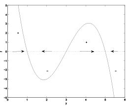
We see that y1 = 1 is stable, y2 = 3 is unstable, and y3 = 5 is stable.
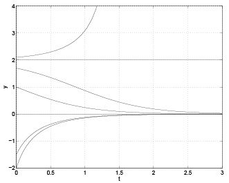
(C). The sketch is given below:
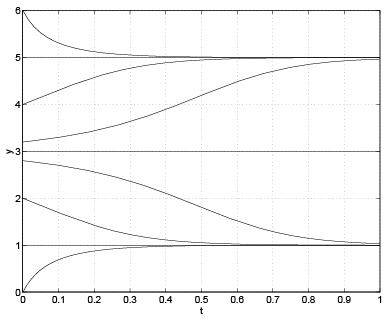
Asymptotic behavior for y as t → ∞ depends on the initial value of y:
- If y(0) < 1, then y(t) → 1,
- If y(0) = 1, then y(t) = 1;
- If 1 < y(0) < 3, then y(t) → 1;
- If y(0) = 3, then y(t) = 3;
- If 3 < y(0) < 5, then y(t) → 5;
- If y(0) = 5, then y(t) = 5;
- if y(t) > 5, then y(t) → 5.
Stability: is not only stable or unstable.
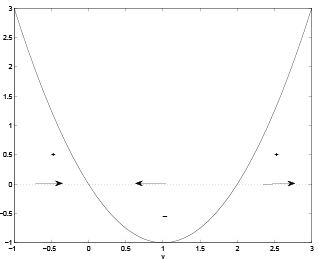
Example 3. For y′ = y2 , we have only one critical point y1 = 0. For y < 0, we have y′ > 0, and for y > 0 we also have y′ > 0. So solution is increasing on both intervals. So on the interval y < 0, solution approaches y = 0 as t grows, so it is stable. But on the interval y > 0, solution grows and leaves y = 0, and it is unstable. This type of critical point is called semi-stable. This happens when one has a double root for f (y) = 0.
Example 4. For equation y′ = f (y) where f (y) is given in the plot
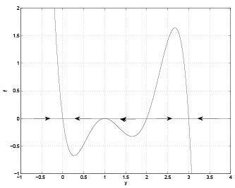
(A). Identify equilibrium points;
(B). Discuss their stabilities;
(C). Sketch solution in y − t plan;
(D). Discuss asymptotic behavior as t → ∞.
Answer. (A). y = 0, y = 1, y = 2, y = 3 are the critical points.
(B). y = 0 is stable, y = 1 is semi-stable, y = 2 is unstable, and y = 3 is stable.
(C). The Sketch is given in the plot:
(D). The asymptotic behavior as t → ∞ depends on the initial data.
- If y(0) < 1, then y → 0;
- If 1 ≤ y(0) < 2, then y → 1;
- If y(0) = 2, then y(t) = 2;
- If y(0) > 2, then y → 3.
Application in population dynamics: let y(t) be the population of a species.
Typically, the rate of change in the population depends on the population y, at any time t.
This means y′(t) typically does NOT depend on t, and we end up with autonomous equations.
Model 1. The simplest model is the exponential growth, with growth rate r:
y′ (t) = ry.
If initially there is no life, then it remains that way. Otherwise, if only a very small amount of population exists, then it will grow exponentially.
Of course, this model is not realistic. In natural there is limited natural resource that can support only limited amount of population.
Model 2. The more realistic model is the “logistic equation”:
 = (r − ay)y.
or
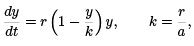
r = intrinsic growth rate,
k = environmental carrying capacity.
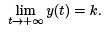
critical points: y = 0, y=k. Here y = 0 is unstable, and y = k is stable.
If 0 < y(0) < k, then y → k as t grows.
If y(0) > k, then y → k as t grows.
Im summary, if y(0) > 0, then
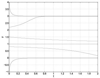
Model 3. An even more detailed model is the logistic growth with a threshold:
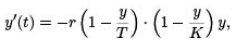
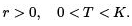
We see that there are 3 critical points: y = 0, y = T , y = K , where y = T is unstable, and y = 0, y = K are stable.
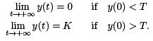
Let y(0) = y0 be the initial population. We discuss the asymptotic behavior as t → +∞.
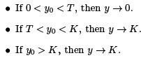
We see that y0 = T work as a threshold. We have
Some populations follow this model, for example, the some fish population in the ocean. If we over-fishing and make the population below certain threshold, then the fish will go extinct.
FAQs on Linear Ordinary Differential Equations of First and Second Order - 2 - Physics for IIT JAM, UGC - NET, CSIR NET
| 1. What is a linear ordinary differential equation of first order? |  |
| 2. How can we solve a linear ordinary differential equation of first order? | |
| 3. What is a linear ordinary differential equation of second order? | |
| 4. How can we solve a linear ordinary differential equation of second order? | |
| 5. What are the applications of linear ordinary differential equations in physics? | |

|
4.63/5 Rating |

|
Dec 23, 2024 Last updated |

|
Explore Courses for Physics exam
|
|
CSIR NET
,Sample Paper
,CSIR NET
,Previous Year Questions with Solutions
,Summary
,UGC - NET
,Linear Ordinary Differential Equations of First and Second Order - 2 | Physics for IIT JAM
,Semester Notes
,Objective type Questions
,ppt
,UGC - NET
,mock tests for examination
,shortcuts and tricks
,Exam
,Viva Questions
,CSIR NET
,UGC - NET
,Linear Ordinary Differential Equations of First and Second Order - 2 | Physics for IIT JAM
,Important questions
,Extra Questions
,study material
,MCQs
,past year papers
,video lectures
,Linear Ordinary Differential Equations of First and Second Order - 2 | Physics for IIT JAM
,practice quizzes
,Free
;


Linear Ordinary Differential Equations of First and Second Order - 2 Free PDF Download
Importance of Linear Ordinary Differential Equations of First and Second Order - 2
Linear Ordinary Differential Equations of First and Second Order - 2 Notes
Linear Ordinary Differential Equations of First and Second Order - 2 Physics Questions
Study Linear Ordinary Differential Equations of First and Second Order - 2 on the App
|
© EduRev
|
Education Revolution
|


|


