Stagflation (Part - 2) - Fiscal Policy, Public Finance | Public Finance - B Com PDF Download
Can Inflation Lower The Unemployment Rate Permanently?
The policy of deliberately stepping up inflation probably would lower the unemployment rate— temporarily. People are unemployed because they don’t find the job opportunities of which they are aware sufficiently attractive. If the level of real wages could somehow be increased across the board, all employment opportunities would become more attractive.
Employment would, therefore, increase except for the fact that employers will demand less labour at higher real wage rates. However, when money wages and prices advance together, as they do in a general inflation, real wages don’t actually increase. But workers think they have increased and that will be enough to lower the unemployment rate.
A policy of deliberate inflation makes job opportunities seem more attractive by raising the money wage rate offers of employers. And this is how inflation reduces unemployment. But the higher wage rate offers are only apparently more attractive. Real wage rates do not rise; only money wage rates rise. As long as potential employees don’t realize that the job opportunities they’re now accepting are in reality no better than the opportunities they previously rejected, employment will indeed rise.
Employment will fall back down to its previous level, however, when employees discover what’s happening and realize that inflation is creating the illusion of more attractive wage offers. As they discover that they’ve been “tricked,” employment will decline again and the Phillips curve will now pass through the point of 7 per cent inflation, but with unemployment back at its previous level of 5 per cent. The curve will have shifted upward. No permanent reduction in unemployment will have occurred, but the economy, anyhow, will be undergoing more rapid inflation.
A deliberate policy of pursuing lower unemployment by creating a higher rate of inflation calls for continually increasing the inflation rate so that workers continually accept less than the actual rate of inflation. In this way they can be made continually to overestimate the real value of the money wages these are being offered. We must either continually increase the rate of inflation or assume that employees’ pay exclusive attention to money wage rates and never consider real wage rates.
This is a superficially plausible assumption; we know that few employees consult the most recent changes in the Consumer Price Index before deciding whether a wage offer is adequate. They look at money wage rates, in other words. But they also learn after a while that their wages buy less and adjust their perception of the wage rate’s real value.
An extreme example will make the point. In 1952 or so workers in USA stood in line for jobs at manufacturing firms offering $ 2 an hour. In 1982 or so manufacturers can find almost no one who will accept employment at that wage.
Employees do know, even if they’ve never heard of price indices, that $ 2 is a much lower hourly wage today than it was thirty years ago. Policy cannot be constructed on the assumption that workers will be permanently fooled; people do learn from experience and the simultaneous existence of high employment with very rapid inflation in the early 1970s through 1980s ought to be sufficient evidence that people have learned. When they begin to assume continued inflation, they no longer suffer from the illusion that money wages and real wages are the same thing.
But now suppose that the government discerns the error of its ways and regrets its policy initiative. Unemployment is back at the old 5 per cent level but inflation is now progressing at 7 per cent per year. The government, therefore, decides to reverse its policy and get inflation down to 3 per cent again. So it eases up on the fiscal monetary stimulus it has been applying. Monetary demand will now stop increasing so rapidly, producers will be unable to sell at the prices they had anticipated, inventories will mount, production will be curtailed, and unemployment will rise.
Eventually, sellers will learn not to expect such a rapid rise in prices, they will adjust downward the prices they ask and the prices they offer to pay for inputs, sales will revive, inventories will decline, production will start up again, and unemployment will fall. But that won’t all happen within a week or even a month. The higher unemployment that will result from an attempt to slow down the rate of inflation will be temporary; but temporary can be a long time.
The cost of letting inflation get out of hand may be very high indeed. It will, therefore, be proper to be warned against confusing cause and effect and assuming that since high employment generates inflation, more inflation will generate higher employment.
Critical Evaluation:
It may, however, be emphasized that not all economists are willing to accept the concept of the Phillips Curve and the empirical evidence is still the subject of too much debate. Many economists are definitely unhappy about an explanation of inflation which says very little about monetary conditions. Even if Phillips relation does exist, they feel, it does not necessarily imply that it will usefully lend itself to macroeconomic decision-making. According to them changes in prices are at least as important as unemployment in determining changes in the wage rate.
This is neglected in the Phillips Curve. The ‘money illusion’ of workers as suggested by Keynes is largely absent in today’s bargaining because wage earners will do their utmost to retain their share of national income, if the same has been eroded by rising prices. Economists question whether the curve is stable and whether the trade-off that it specifies actually exists. Implicit in this challenge to the Phillips Curve is an alternate theory of how workers behave.
We have seen that Phillips model is based on the notion of money illusion in the labour market—which acts to befool the workers into accepting lower real wages. But those who are opposed to the theory of money illusion argue that labour is less gullible, and that expectations about wages change more quickly. If expectations about real wages change quickly and wages are revised accordingly, there is, then, little likelihood of the trade-off between inflation and unemployment.
Economists like Milton Friedman and Edmund Phelps have mounted one of the theoretical attacks on the Phillips Curve property of trade-off between inflation and unemployment. Basically they hold the view that overtime workers adjust their money wages in line with their real wages and hence, they argue, that there is no long-run trade-off as specified by Phillips Curve.
There is room in this theory, however, for short-run trade-offs similar to those specified by the Phillips Curve. This view is called ‘the accelerationist theory’—it admits that in the short-run an unanticipated increase in the rate of inflation will lower real wages and reduce unemployment, but in the long-run there may be no trade-off as shown in the Fig. 33.3:
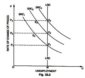
In this Figure unemployment will move along with the short-run Phillips Curve, SRC1, from point E1 to point E2 (with an increase in price from P1 to P2). However, as soon as the workers realize that high price at P2 is a fact of life, they adjust money-wage demands upwards to restore real wages to the level formerly held at E2. The resultant increase in real wages over those prevailing at E2 moves employment back to E3 on SRC2, which is the same level of unemployment which existed previously, with one difference that at E3 the rate of increase in money-wages and prices is higher than it was before.
The long-run Phillips Curve LRC is thus vertical at point N, and is taken to be the natural rate of unemployment, as determined by normal frictions in the labour market. A subsequent effort to reduce unemployment with further inflation by raising prices from P2 to P3 may again be successful in the short-run, causing the rate of unemployment to decline along SRC2 to E4 from E3.
But if labour once again comes to know of it and adjusts the wages over time, the impact of inflation on employment will fall so that even if the second dose or increase in inflation equals the first (P1P2 = P2P3), that is, the distance from E5 to E3 the distance from E3 to E 1—the second reduction in employment for a given acceleration in the rate of inflation (E5– E3 = E3– E1) will be reduced. The distance from E4 to E5 will be less than the distance from E2 to E3.
This clearly explains that if prices are rising steadily over a long period of time, wage increases will not lag behind increase in prices as labour becomes fully aware of price increases and include escalator clauses into contracts. Thus, the reduction in real wages, which is the means by which the unemployment rate is reduced as production expands, no longer takes place. Hence, the trade-off between unemployment and inflation disappears in the long-run.
Unemployment will remain at, what is called natural rate (N) as the workers learn to fully anticipate the reduction in real wages implied by inflation. Friedman has argued that in recent years this level of natural unemployment has increased in western economies like UK, USA on account of technological advances that have reduced the demand for labour. This factor, combined with the entry of a large number of young people and previously unemployed women into the job market, has resulted in large-scale unemployment of workers which the economy cannot absorb, even though the economy may be at full employment.
The choices are, therefore, either to accept the fact of normal or natural unemployment rate over the long- run in excess of four per cent or to provide training programmes and effect efforts to increase job mobility by improving the flow of information about job vacancies and available labour. The result would be to shift the vertical line at N (natural rate of unemployment) to the left.
Optimal Trade-off:
The opposing views on the trade-off lead to opposing policies toward the control of inflation and unemployment. Those who deny the possibility of a lasting trade-off and argue that there is only one equilibrium rate of unemployment conclude that the appropriate public policy is one of hands off that allows the unemployment rate to gravitate to this equilibrium of natural rate. But those who argue that there is a steady state trade-off are led to a ‘hands on ‘policy.
They argue, we can have a lower rate of unemployment if we are willing to accept a higher rate of inflation, and we can have this tradeoff not merely on a temporary basis. This group believing that there is indeed a durable trade-off is then confronted with the question of what the optimal trade-off is?
The approach to this kind of problem involves cost-benefit analysis. To choose the benefit of less inflation involves the cost of more unemployment, or to choose the benefit of less unemployment involves the cost of more inflation. The objective should be to attain a position such that any departure from it will add more to costs than to benefits.
Although we potentially have a wide range within which a trade-off may be selected, the one that will be optimal on a cost-benefit basis will be one that accepts, if necessary, relatively high inflation as the price of relatively low unemployment. From this viewpoint, the question in time of inflation is not how do we end the inflation but rather how do we learn to live with it, because we can devise methods of living with inflation but we cannot devise methods of living with unemployment. Opinion as to the trade-off that will provide the best balance between the twin evils of inflation and unemployment is probably shifting now-a- days towards the acceptance of the cost of relatively higher inflation in order to secure the benefit of relatively smaller unemployment.
A Modified Phillips Curve:
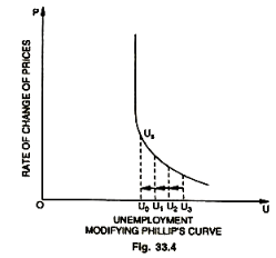
While Friedman’s analysis is convincing, the fact remains that a substantial body of empirical evidence exists showing that something like the traditional Phillips Curve obtains over long periods of time in industrialized countries. A theory of the Phillips Curve has been developed recently which suggests a compromise between the traditional view and the accelerationist view. The Fig. 33.4 shows a modified Phillips Curve consisting of a positively sloped lower portion suggesting a trade-off between unemployment and inflation at relatively high levels of unemployment and a vertical line suggesting no trade-off at low levels of unemployment.
This view was put forward by J.E. Tobin in 1972. In effect Tobin’s analysis suggests that at high levels of unemployment (U3), accelerating inflation will reduce involuntary unemployment (U3 to Uo). As unemployment falls, however, the trade-off disappears and changes in the rate of inflation become an ineffective means of affecting the level of unemployment. Tobin’s discontinuous Phillips Curve has the advantage that it does not imply the troublesome hypothesis that unemployment rates slightly above the natural or critical rate of unemployment will trigger an even-accelerating deflation. Friedman’s vertical Phillips Curve does carry this implication.
Moreover, other refinements to the Phillips Curve are to be seen from the fact that wage decisions are based on previous levels and wage bargainers do not change their demands because of the current movements in economic indicators.
Again, the degree of non-linearity between changes in the wage rate and unemployment is an empirical question with needs further examination. Profits have often been suggested as another important determinant of the change in wages. This point needs serious consideration. Hence, the validity of Phillips Curve is obviously to be accepted subject to these limitations and refinements.
Causes of Stagflation—Keynesian, Monetary and Supply Side Perspectives:
Economic strength of labour unions backed by various types of labour acts in different developed and developing countries of the world giving encouragement to unionism and collective bargaining, accompanied by the substantial market power of big business and multinationals—because of the nature of modern technology resulting in lower unit production costs—a few large firms dominate many major manufacturing units. Their big size enables these industrial giants to exert a degree of control over their prices that would be impossible in an otherwise thorough going competitive economy, thereby, allowing them to some extent to pass cost increases on to their customers.
These factors followed by Employment Act in different countries under which governments are assuming greater responsibility for maintaining high employment levels-through the use of its monetary, fiscal and related powers followed by another element called imported inflation particularly after the rise in oil prices in 1973 by international oil cartel called OPEC affecting the domestic prices of national economies are the important causes that gave rise to the worldwide phenomenon of stagflation.
Causes—Keynesian Perspective:
According to Keynesians the stagflation has been on the increase because:
(a) OPEC oil price increases caused a large ‘cost shock’ that worsened the unemployment-inflation trade-off
(b) Unions caused cost-push inflation;
(c) Inflationary expectations arose and caused further inflation;
(d) A changed composition of labour force caused higher levels of unemployment.
Keynesians argue that cost shocks, such as the exhorbitant increase in oil prices over the decade of the 1970s, caused supply or cost-push inflation. They contended that inflation is caused either by rising aggregate total demand or by falling aggregate total supply and the resultant increases in resource prices lead to high costs for producers. This shifted the aggregate supply curve for the economy backward (higher cost of resources result in backward shifts of supply).
Cost-push inflation, as per this view, was also caused by the unions who demanded and received wage increases that exceeded the productivity gains. When wages rise faster than productivity, the later defined as output per worker-hour, than labour and total costs to the firm rise; supply curves shift backward, and product prices increase. Again, once inflation sets in people expect it to continue or even rise.
They decide to buy products immediately rather than wait because they expect that the prices will be even higher in the near future. This creates increased current aggregate demand which lead to further increase in prices. Along with this even the unions begin to build expectations of inflation and start asking for higher wages; as such inflationary expectations can produce both demand and supply inflation which cause the Phillip’s curve to rise or shift rightwards.
This tendency is further reinforced by the changed composition of the labour force—more women, youth and teenagers. Women teenagers had higher unemployment rates than the average and as the labour force composition became more heavily weighted towards them, the average went up. They added extra income to the family and spent more adding to inflation and causing shifts in Phillip’s curve.
Supply Side Perspective:
Supply side economists partially explained the phenomenon of stagflation of the 1970s through:
(a) Government taxes,
(b) Cost increasing government regulations,
(c) Increases in military spending,
(d) Reduced government transfer payments,
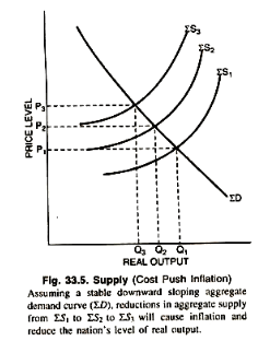
Supply side economists—so named because they focus their attention on factors than affect aggregate supply rather than aggregate demand. They quote different forces that those cited by the Keynesians for causing upward shift in Phillip’s Curve. One of these is the increased government regulations during the late 1960s and 1970s.
These regulations increased the costs of producing goods and services, which in turn, reduced aggregate supply and caused the price level to rise. Figure 33.5 explains this supply curve position and the movement from ∑S1 to ∑S2 to ∑S3 on account of different causes. According to supply side economists the ‘tax wedge’ had increased during the 1970s. The tax wedge is simply that part of product prices that covers the various taxes that the firm was mandated to pay to government.
A major source of this increased tax wedge was the higher social security tax that firms had to pay for their employees. A higher tax wedge leads to higher cost, reduced supply and higher prices. A higher tax or tax bracket produced higher real tax burdens in the society reduced incentives to work, save and invest—reduced the value of work relative to the value of leisure—an hour of work now had a lower after tax return—all this meant according to supply side reduced work efforts.
Increased transfer payments by government reduced incentives on the part of recipients to work and seek training. All this combined led to less work, saving, investment, capital formation, reduced technological advances and caused productivity to decline resulting in backward shifts in the aggregate supply curve and a worsening of trade-off between unemployment and inflation.
The Monetarist Perspective:
According to monetarists, the long-run Phillip’s curve is vertical at the ‘natural rate of unemployment. The natural rate of unemployment is the rate which prevails according to the frictions in the labour market. According to them there is no trade off between unemployment and inflation (U and I) in the long-run. The only trade-off is between less unemployment than the natural rate today versus more than that rate tomorrow.
Thus, Keynesian looked at stagflation as outward or upward shift to the Phillip’s curve caused by cost shocks, wage-push inflation, inflationary expectations and the changing composition of the labour force. The supply side economists instead blamed government actions, government regulations, increased tax wedge, increased transfer payments and improper monetary policy and aggregate demand management.
The monetarists also blamed the government but held the Federal Reserve in USA improper monetary policy primarily responsible for stagflation. The monetary policy followed by the central bank according to monetarists was based on erroneous Keynesian view of a stable long-run Phillip’s relationship between U and I. For monetarists, long-run Phillip’s curve is perfectly vertical at the ‘natural rate of unemployment, as already shown in previous pages.
Policy Alternatives—Stopping Stagflation:
Because the Keynesians, the Supply Side Economists, and Monetarists view the causes of stagflation differently, it is, therefore, no wonder that they disagree on what ought to be done or on the proper policy alternative to stop stagflation and also to keep it from recurring again or even continuing for a long period.
Keynesians proposed implementing:
(a) Tight money policy,
(b) Expansionary fiscal policy,
(c) Incomes policy.
Incomes policy consists of government actions that limit monetary wage, rent, interest and profit increases thereby reducing cost-push inflation. This type of policy will break inflationary expectations. Supply side economists advocated tax cuts to stimulate work efforts, savings, investment and economic growth, cut the tax wedge, increased incentives to work, save and invest that generally promote economic growth and total supply in the economy.
According to Monetarists the best way to stop stagflation and bring it under control is to increase the money supply at a steady rate of 4 to 6 per cent annually upholding the monetary’ rule? However, it is said that the macroeconomics policies in the early 1980s were the mixture of supply side, monetarist and even disguised Keynesian policies, so it is difficult to sort out and to say with confidence which policy worked and which failed even under Reagan administration in USA. Despite, following these policies separately and jointly the confusion and turmoil on economic front in USA are still there and stagflation continues to be a tormenting problem even at the end of 1980s, to which there appears to be no easy solution.
Fiscal and Monetary Policy Mix:
The very concept of a fiscal and monetary policy mix as advocated by Nobel Prize Winner Professor James Tobin (1981) presupposes that governments and central banks jointly enjoy some freedom of choice, that they can set fiscal and monetary instruments independently one from the other to control situations like inflation, deflation or more appropriately speaking stagflation.
As usual in macroeconomics it is necessary to distinguish between short and long runs. In short- run, fluctuations of business activity, the policies affect aggregate demand, production, unemployment and capacity utilization, interest rates and prices. In the long-run, when output is constrained by available resources and their productivity rather than by demand, the policy mix affects the accumulation of capital, the path of economic growth and the trend of prices.
Therefore, Professor James Tobin plead that these days any economist who takes seriously the theory of short-run demand management, stabilization policy, must begin by showing awareness of fashionable contemporary theories that the economy is not manageable by government intervention alone, that systematic demand policies are necessarily ineffective, that business cycles are the tracks (paths) of moving equilibria.
These are the propositions of self-styled new classical macroeconomics—logically derived from marrying old fashioned competitive price clearing markets to new-fangled rational expectations. This elegant revival of neoclassical economics appeals to professional theorists and sharpens their tools—but the explanations and the attempts that it makes for controlling problems like stagflation are still found wanting in many ways.
The problem is that the two most important short-run macroeconomic targets of inflation and unemployment have to be contained to acceptable rates by suitable choice of the fiscal and monetary mix. An analysis of the welfare macroeconomics of the policy mix was a contribution of the neoclassical and neo-Keynesian synthesis proposed by American economists led by Professor Paul Samuelson in the 1950s and 1960s. Professor Tobin developed an idea called “common funnel theorem”.
It says that it is the total aggregate demand, not the distribution of its resources, that determines the combination of outcomes for unemployment and inflation. It is the total size of a demand management package, whatever is its fiscal-monetary mix, that helps to determine the combination of output and employment results, on the one hand, and nominal wage and price movements on the other.
Relative to these two objectives of U and I monetary and fiscal instruments are not independent, collinear. But this ‘common funnel proposition’ as advocated by Prof. Tobin is at the most a strong first approximation, like most macroeconomic assertions and no more than that. Professor Tobin is of the view that no useful purpose will be served by a net withdrawal of demand stimulus but for a different mixture of medicines, less fiscal tonic and more monetary elixir may be in order.
The phenomenon of stagflation being very complicated in nature cannot be controlled except through a judicious policy mix of measures particularly monetary and fiscal. Even this policy mix has to be varied according to the situation and the nature of the economy and also keeping in mind the fact whether the policy mix is being adopted in a closed economy or in an open economy.
Since stagflation has become a global problem the adoption of a suitable policy mix on a global scale is likely to be the main precondition for solving the problem. The mix of tax rates, government spending and monetary policy will have effects on the price level and on the rate of inflation at any given level of economic activity. Much more attention than in the past, therefore, needs to be paid to the particular mix of these measures.
The relative effects on the price level and on output—of taxation, of government spending. and monetary policy are more or less clear by now. For example, so long as a government is concerned to reduce the rate of inflation it should reduce tax rates whenever possible and be prepared simultaneously to allow nominal interest rates to rise to maintain the desired level of activity. If the aim of the government is to maintain a given level of activity with less inflation it should try to cut taxes and sell more bonds to the public.
Regarding government spending the conclusions are less clear-cut. In general, however, those forms of government spending that are wasteful in the sense that the sources they employ could be better employed elsewhere—should be cut. But there is no general case for cutting government expenditure merely on the expectation that to do so will straightaway reduce the rate of inflation. As a matter of fact some forms of government spending specially those involving subsidy—may be at least as effective in reducing cost-push inflation as are many forms of tax reductions.
The most appropriate policy mix in a closed economy where the aim is to reduce the price level and the possible rate of inflation—is to keep taxes low, especially those that are likely to have cost effect and to sell enough attractive financial assets to the public to keep down the growth of the money supply. This policy mix of measures will have to be varied in different phases of the cycles or in an economic activity depending upon the nature of an economy.
In an open economy it is unwise to use the exchange rate as an additional instrument. It is much more defensible to regard it as simply one of the channels through which an appropriate setting of the monetary and budgetary instruments will operate in bringing about the desired combination of employment and inflation. In an open as well as closed economy, a government should apply the rule of tight monetary policy so long as inflation is too rapid and using expansionary budgetary measures so long as unemployment is so low.
The direction in which macroeconomic instruments should be changed with a view to affecting the main aims of macroeconomic policy should be such that each instrument is directed at influencing the objective for which it is most appropriate. When high unemployment and high scales of inflation occur together (stagflation)—the appropriate assignment of instruments to objections becomes the touch stone of a well-designed macroeconomic policy.
In short, the adoption of timely and the right type of macroeconomic policy mix would enable governments to avoid many sort of mistakes that they have made in recent years, which have intensified stagflation— though such a policy mix will not be a panacea for all sorts of economic troubles.
J.M. Keynes addressed his policy prescriptions in the General Theory in the 1930s for advanced economics in depths of depression. Similarly, a new school of thought called Supply Side Economists’ (Neo- classicals) direct their policy prescriptions to remedy the malady of ‘stagflation’—a phenomenon they feel peculiar to developed economies (though developing economies are no exception). Needless, however to say that even they had little success to control the phenomenon of stagflation.
|
37 videos|35 docs|15 tests
|
FAQs on Stagflation (Part - 2) - Fiscal Policy, Public Finance - Public Finance - B Com
| 1. What is fiscal policy and how does it relate to stagflation? |  |
| 2. How can fiscal policy be used to combat stagflation? | |
| 3. What are the potential drawbacks of using fiscal policy to combat stagflation? | |
| 4. Can fiscal policy alone solve the problem of stagflation? | |
| 5. How does public finance play a role in managing stagflation? | |

|
4.86/5 Rating |

|
Dec 23, 2024 Last updated |

|
Explore Courses for B Com exam
|
|
shortcuts and tricks
,study material
,Public Finance | Public Finance - B Com
,Public Finance | Public Finance - B Com
,Objective type Questions
,Free
,Exam
,Stagflation (Part - 2) - Fiscal Policy
,Extra Questions
,Viva Questions
,Semester Notes
,Summary
,MCQs
,Previous Year Questions with Solutions
,Stagflation (Part - 2) - Fiscal Policy
,Stagflation (Part - 2) - Fiscal Policy
,ppt
,Sample Paper
,mock tests for examination
,practice quizzes
,past year papers
,video lectures
,Important questions
,Public Finance | Public Finance - B Com
;


Stagflation (Part - 2) - Fiscal Policy, Public Finance Free PDF Download
Importance of Stagflation (Part - 2) - Fiscal Policy, Public Finance
Stagflation (Part - 2) - Fiscal Policy, Public Finance Notes
Stagflation (Part - 2) - Fiscal Policy, Public Finance B Com Questions
Study Stagflation (Part - 2) - Fiscal Policy, Public Finance on the App
|
© EduRev
|
Education Revolution
|


|


