Short Run & Long Run Cost Curves - Cost Function Analysis, Business Economics & Finance


In this article we will discuss about Cost in Short Run and Long Run.
Cost in the Short Run
In economics cost is often classified by its behaviour with respect to changes in output rather than by its function. In the short run some inputs are fixed (cannot be varied), so costs associated with those fixed inputs must be incurred regardless of the level of output. Other costs vary with output. The sum of all such costs - fixed and variable, explicit and implicit - for a given period is the short-run total cost (STC).
For analytical simplicity we usually divide short-run costs into two broad categories:
- Fixed cost (TFC) - costs that do not vary with output in the short run (for example, rent, depreciation, license fees, interest on loan). These are unavoidable while the firm continues to operate.
- Variable cost (TVC) - costs that vary with the level of output (for example, raw materials, wages of casual workers, electricity tied to production).
Short-Run Total Cost Curve
A typical short-run total cost curve (STC) shows the total cost of production for each output level when one or more inputs are fixed. When output is zero, STC is positive because fixed costs remain. The TFC curve is a horizontal line (since fixed cost does not change with output). The TVC curve starts from the origin because when output is zero variable cost is zero.
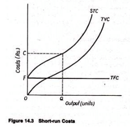
Variable cost and total cost increase with output. Often TVC and STC increase first at a decreasing rate, and then at an increasing rate; this pattern is explained by the Law of Variable Proportions (also known as the law of diminishing marginal returns) acting on the variable factor(s).
Average and Marginal Cost in the Short Run
Analysing average and marginal costs provides clearer insight into cost behaviour.
Average Fixed Cost (AFC)
AFC = TFC / Q
Because TFC is constant, AFC falls as output Q increases. Graphically AFC is a rectangular hyperbola that approaches zero as output becomes very large.
Average Variable Cost (AVC)
AVC = TVC / Q
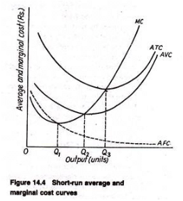
The typical AVC curve is U-shaped: it falls initially, reaches a minimum at some output (call it Q2), and then rises as diminishing marginal returns set in.
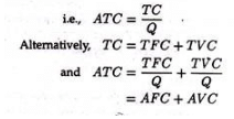
Average Total Cost (ATC)
ATC = TC / Q = AFC + AVC
The ATC curve is also U-shaped. Because AFC keeps falling as output rises, the minimum point of ATC (call it Q3) occurs at a larger output than the minimum point of AVC. The vertical distance between ATC and AVC at any output equals AFC; as output increases, AFC shrinks and AVC and ATC converge.
Short-Run Marginal Cost (SMC or MC)
MC = ΔTC / ΔQ
Marginal cost reflects the change in total cost that results from producing an additional unit of output when variable inputs change. The typical MC curve falls at first (due to increasing marginal returns from better utilisation of variable inputs), reaches a minimum at some output Q1 (which is usually less than Q2 and Q3), and then rises because of diminishing marginal returns.
Important relationships:
- When MC is below AVC (or ATC), the respective average curve falls.
- When MC is above AVC (or ATC), the respective average curve rises.
- MC intersects AVC and ATC at their minimum points.
Short-Run Cost Functions
All important short-run cost relations can be summarised algebraically.
Total cost function:
TC = k + f(Q) where k is the total fixed cost (a constant) and f(Q) is the total variable cost as a function of output Q.
Average total cost:
ATC = k/Q + f(Q)/Q = AFC + AVC
Since k is constant and Q increases, AFC = k/Q falls as Q increases.
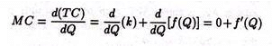
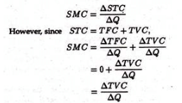
Because MC is the change in TVC with respect to Q, one can express MC equivalently as the derivative of TVC with respect to Q (continuous case) or as the discrete increment ΔTVC/ΔQ:
- MC = f'(Q) = ΔTVC/ΔQ
- Fixed cost does not affect marginal cost. Business decisions that depend on marginal analysis therefore do not depend on sunk fixed costs.
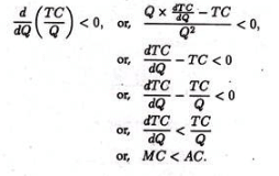
Relation between MC and AC
When AC is falling, marginal cost must be below average cost; when AC is rising, marginal cost must be above average cost. This leads to the general rule that MC crosses AC at AC's minimum.
Cost Elasticity
The cost elasticity measures the responsiveness of total cost to a small change in output. It can be written as the ratio of marginal cost to average cost:
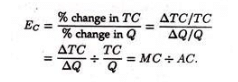
Thus, cost elasticity = MC / AC. This concept is useful for understanding percentage changes in cost relative to percentage changes in output.
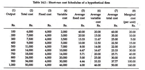
A numerical table (for example Table 14.2) typically illustrates: AFC declines with output; AVC and ATC fall then rise; MC falls then rises and is below average curves when they are falling and above when they are rising.
Long-Run Costs: The Planning Horizon
The long run is a planning period in which all factor inputs are variable. There are no fixed inputs in the long run (except exogenous aspects such as factor prices or technology, which we typically hold constant for the analysis). Therefore, the firm can choose its scale of operation - the size of plant or capital stock - and select the least-cost combination of inputs for each output level.
Derivation of Long-Run Cost Schedules from a Production Function
Assume factor prices are given and the production function is known. The firm's manager chooses, for each output level, the combination of labour and capital that minimises cost at the given factor prices. The locus of these least-cost combinations is the firm's expansion path.
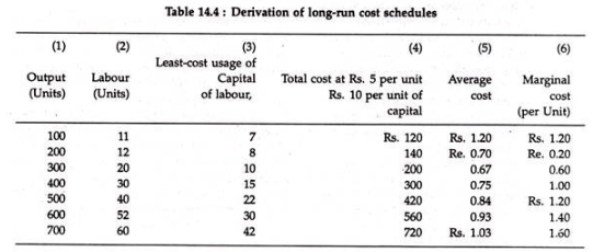
For illustration, suppose labour costs Rs. 5 per unit and capital costs Rs. 10 per unit. An expansion path table might show, for each output level, the optimal labour and capital combination and the resulting total cost at those factor prices. From the total cost column we can compute:
- Long-run average cost (LAC) = Total cost / output.
- Long-run marginal cost (LMC) = Δ total cost / Δ output.
Typically LAC first falls, reaches a minimum, and then rises; LMC falls then rises, and LMC intersects LAC at LAC's minimum. Numerically, if producing 300 units requires 20 units of labour and 10 units of capital and the resulting total cost is Rs. 200, then average cost is Rs. 200/300 ≈ Rs. 0.667 per unit. The marginal cost between two output levels is the change in total cost divided by the change in output (for example, MC between 100 and 200 units = (TC@200 - TC@100)/(200 - 100)).
Expansion Path and the Long-Run Total Cost Curve
Graphically, draw isoquants for different output levels and isocost lines for the given factor-price ratio. The tangency points of isoquants and isocosts give the least-cost input combinations for each output. The expansion path joins these tangency points.
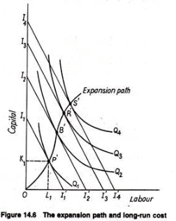
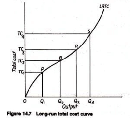
Mapping least-cost points into output-cost space gives the long-run total cost (LRTC) curve. Each point on LRTC shows the minimum cost of producing the corresponding output when all inputs can be varied.
Because fixed costs do not exist in the long run, the LRTC curve starts from the origin. Its slope represents LMC; typically LRTC increases at a decreasing rate up to some point and then at an increasing rate thereafter, reflecting falling then rising LMC.
Long-Run Average and Marginal Costs
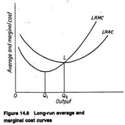
Long-run average cost (LAC) is defined as:
LAC = LRTC / Q
Long-run marginal cost (LMC) is defined as:
LMC = ΔLRTC / ΔQ
Graphically, LAC is typically U-shaped and LMC intersects LAC at LAC's minimum. The same logic that explains the MC-AC relationship in the short run applies in the long run: if LMC < LAC, adding output reduces LAC; if LMC > LAC, adding output increases LAC; equality holds at the minimum point.
As Maurice and Smithson summarised, when marginal cost is less than average cost, each additional unit adds less than the average and hence average falls; when marginal cost is greater, average rises; therefore LMC must equal LAC at LAC's minimum.
The Shape of the LAC: Economies and Diseconomies of Scale
The long-run average cost curve's shape reflects advantages and disadvantages of expanding firm size - these are called economies and diseconomies of scale.
Economies of Scale (Decreasing LAC)
Factors that give rise to economies of scale include:
- Greater specialisation of resources - larger firms can divide tasks more finely among workers and machines.
- More efficient utilisation of equipment - large plants can use costly machines more fully and spread fixed costs per unit over a larger output.
- Reduced unit costs of inputs - bulk purchasing often yields discounts; unit construction costs (per square foot) may decline with scale.
- Utilisation of by-products - large firms can use or sell by-products that small firms might waste (for example, molasses or bagasse in sugar production).
- Growth of auxiliary facilities - large-scale production can attract or support better transport, warehousing, repair and marketing services.
Diseconomies of Scale (Increasing LAC)
At sufficiently large scales, disadvantages may arise that increase average cost. Principal reasons include:
- Management and coordination problems - as organisations grow, decision-making becomes slower, communication costs rise and the marginal productivity of management may fall.
- Competition for scarce resources - large firms may bid up wages or input prices in local labour or input markets, raising unit costs.
The combined effect of economies and diseconomies determines the overall shape of LAC. There are three commonly discussed forms:
- LAC slopes up quickly after a small output (when diseconomies dominate early) - see Panel A.
- LAC slopes down or stays flat over a wide range (large economies of scale) - typical of natural monopolies - see Panel B.
- LAC is largely flat for a broad range of output (constant returns to scale over that range) - see Panel C.
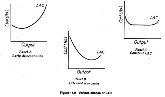
In practice many industries show a mixture: initial falling LAC (economies), a long flat region (constant returns), and rising LAC at very large scale (diseconomies).
Average Cost in the Long Run: The Envelope (Smooth) Case
In the short run the firm must operate with a fixed plant and so faces a particular short-run average cost curve (SAC). If the firm is planning, it can choose among many possible plant sizes; each plant has its own SAC (typically U-shaped). The long-run average cost curve (LAC) is the lower envelope of all possible SAC curves: for each output level the firm picks the plant whose SAC gives the lowest average cost.
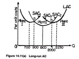
For example, if three plant sizes I, II and III have SAC curves that are lowest in different ranges, the LAC will follow the lowest portions of these SACs: Plant I's SAC for low output, Plant II's SAC for intermediate output, and Plant III's SAC for high output. If there is a continuum of plant sizes available, the envelope becomes smooth. Samuelson describes the long‐run choice as selecting the plant that yields the lower envelope curve; with many possible choices the LAC is a smooth curve.
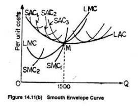
In the smooth envelope case, one can derive LMC from LAC; LMC intersects LAC at its minimum and tends to be smoother than the short-run MC curves associated with individual plants.
Key Concepts and Practical Applications
- Shut-down point: The minimum point of the AVC curve; below this output the firm cannot cover variable costs and should temporarily shut down in the short run.
- Break-even point: The minimum point of the ATC curve; at this output the firm covers both fixed and variable costs and earns zero economic profit.
- Policy and managerial use: Understanding these cost curves helps managers decide plant size, pricing at different output ranges, and whether to expand or contract production. For governments and regulators, knowledge of LAC shapes aids decisions on natural monopoly regulation and industrial policy.
- Marginal analysis: Since many decisions are governed by marginal criteria (e.g., produce where MR = MC), recognising that MC is independent of sunk fixed cost is crucial: sunk costs should not affect marginal decisions.
Summary (optional): Short-run cost analysis distinguishes fixed and variable costs and gives rise to AFC, AVC, ATC and MC curves, with MC intersecting AVC and ATC at their minima. In the long run all inputs are variable; the firm chooses least-cost input combinations yielding the expansion path and the long-run total and average cost curves. The LAC reflects economies and diseconomies of scale and is the lower envelope of short-run average cost curves.
FAQs on Short Run & Long Run Cost Curves - Cost Function Analysis, Business Economics & Finance
| 1. What is the difference between short run and long run cost curves in cost function analysis? |  |
| 2. How are short run and long run cost curves related to business economics and finance? | |
| 3. How can cost function analysis be applied in business decision-making? | |
| 4. What are some factors that can cause shifts in short run and long run cost curves? | |
| 5. What are some limitations of cost function analysis in business economics and finance? | |