Perfect Competition- 2 | Business Economics for CA Foundation PDF Download
Can a competitive firm earn profits?
In the short run, a firm will attain equilibrium position and at the same time, it may earn supernormal profits, normal profits or losses depending upon its cost conditions. Following are the three possibilities:
Supernormal Profits: There is a difference between normal profits and supernormal profits. When the average revenue of a firm is just equal to its average total cost, a firm earns normal profits or zero economic profits. It is to be noted that here a normal percentage of profits for the entrepreneur for his managerial services is already included in the cost of production. When a firm earns supernormal profits, its average revenues are more than its average total cost. Thus, in addition to normal rate of profit, the firm earns some additional profits. The following example will make the above concepts clear:
Suppose the cost of producing 1,000 units of a product by a firm is ₹ 15,000. The entrepreneur has invested ₹ 50,000 in the business and the normal rate of return in the market is 10 per cent. That is, the cost of self owned factor (capital) used in the business or implicit cost is ₹ 5000/-. The entrepreneur would have earned ₹ 5,000 (10% of ₹ 50,000) if he had invested it elsewhere. Thus, total cost of production is ₹ 20,000 (₹ 15,000 + ₹ 5,000). If the firm is selling the product at ₹ 20, it is earning normal profits because AR (₹ 20) is equal to ATC (₹ 20). If the firm is selling the product at ₹ 22 per unit, its AR (₹ 22) is greater than its ATC (₹ 20) and it is earning supernormal profit at the rate of ₹ 2 per unit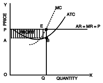
Fig. 18: Short run equilibrium: Supernormal profits of a competitive firm
Figure 18 shows the revenue and cost curves of a firm which earns supernormal profits in the short run. MR (marginal revenue) curve is a horizontal line and MC (marginal cost) curve is a U-shaped curve which cuts the MR curve at E. The firm is in equilibrium at point E where marginal revenue is equal to marginal cost. OQ is the equilibrium output for the firm. At this level of output, the average revenue or price per unit is EQ and average total cost is BQ. The firm’s profit per unit is EB (AR-ATC). Total profits are ABEP. (EB x OQ ; OQ =AB) . Applying the principle Total Profit = TR – TC, we find total profit by finding the difference between OPEQ and OABQ which is equal to ABEP.
Normal profits: When a firm just meets its average total cost, it earns normal profits. Here AR = ATC.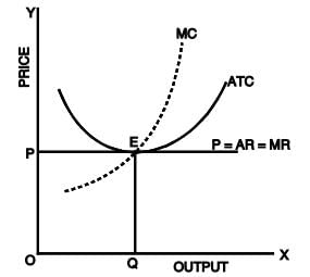
Fig. 19: Short run equilibrium of a competitive firm: Normal profits
The figure shows that MR = MC at E. The equilibrium output is OQ. At this level of output, price or AR covers full cost (ATC). Since AR = ATC or OP = EQ, the firm is just earning normal profits. Applying TR – TC, we find that TR – TC = zero or there is zero economic profit.
Losses: The firm can be in an equilibrium position and still makes losses. This is the situation when the firm is minimising losses. For all prices above the minimum point on the AVC curve, the firm will stay open and will produce the level of output at which MR = MC. When the firm is able to meet its variable cost and a part of fixed cost, it will try to continue production in the short run. If it recovers a part of the fixed costs, it will be beneficial for it to continue production because fixed costs (such as costs towards plant and machinery, building etc.) are already incurred and in such case it will be able to recover a part of them. But, if a firm is unable to meet its average variable cost, it will be better for it to shutdown. This shutdown may be temporary. When the market price rises, the firm resumes production.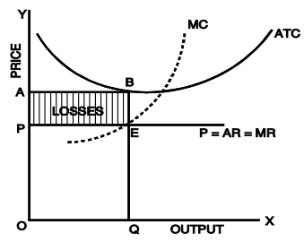
Fig. 20: Short run equilibrium of a competitive firm: Losses
In figure 20, E is the equilibrium point and at this point AR = EQ and ATC = BQ since BQ>EQ, the firm is having per unit loss equal to BE and the total loss is ABEP.
ILLUSTRATION
“Tasty Burgers” is a small kiosk selling Burgers and is a price-taker. The table below provides the data of 'Tasty Burgers’ output and costs in Rupees.
| Quantity | Total Cost | Fixed Cost | Variable Cost | Average Variable Cost | Average Fixed Cost | Marginal Cost |
| 0 | 100 | |||||
| 10 | 210 | |||||
| 20 | 300 | |||||
| 30 | 400 | |||||
| 40 | 540 | |||||
| 50 | 790 | |||||
| 60 | 1060 |
Q1. If burgers sell for ₹ 14 each, what is Tasty Burgers’ profit maximizing level of output? Q2. What is the total variable cost when 60 burgers are produced?
Q3. What is average fixed cost when 20 burgers are produced?
Q4. Between 10 to 20 burgers, what is the marginal cost?
Let us try to solve each of these questions.
First of all it is better to fill the blanks in the Table.
Since the total cost when zero product is produced is ₹ 100, the total fixed cost of “Tasty Burgers” will be ₹ 100/-. We fill the data now:
| Quantity | Total Cost | Fixed Cost | Variable cost | Average Variable cost | Average Fixed Cost | Marginal Cost | MArginal Cost ( Per Unit) |
| 0 | 100 | 100 | - | - | - | - | - |
| 10 | 210 | 100 | 110 | 11 | 10.0 | 110 | 11 |
| 20 | 300 | 100 | 200 | 10 | 5.0 | 90 | 9 |
| 30 | 400 | 100 | 300 | 10 | 3.33 | 100 | 10 |
| 40 | 540 | 100 | 440 | 11 | 2.50 | 140 | 14 |
| 50 | 790 | 100 | 690 | 13.80 | 2.0 | 250 | 25 |
| 60 | 1060 | 100 | 960 | 16 | 1.66 | 270 | 27 |
Now let us answer the questions.
Ans 1: The price of Burger is ₹ 14. Since it is given that “Tasty Burger” is price-taker, it is a perfectly competitive firm. In a perfectly competitive market all the products are sold at the same price, that means AR = MR. In order to find out the profit maximizing level of output, MR should be equal to MC. Here AR = MR = ₹ 14. From the table we can see that MR (14) = MC (14) when 40 burgers are produced. Therefore, the profit maximising level of output of burgers is 40 units.
Ans 2 : The Total Variable Cost at 60 burgers is ₹ 960.
Ans 3: The Average Fixed Cost at 20 burgers is ₹ 5.
Ans 4: Between 10 to 20 burgers, the Marginal Cost is ₹ 9.
Long Run Equilibrium of a Competitive Firm
In the short run, one or more of the firm’s inputs are fixed. In the long run, firms can alter the scale of operation or quit the industry and new firms can enter the industry. In a market with entry and exit, a firm enters when it believes that it can earn a positive long run profit and exits when it faces the possibility of a long-run loss. Firms are in equilibrium in the long run when they have adjusted their plant so as to produce at the minimum point of their long run ATC curve, which is tangent to the demand curve defined by the market price. In the long run, the firms will be earning just normal profits, which are included in the ATC. If they are making supernormal profits in the short run, new firms will be attracted into the industry; this will lead to a fall in price (a down ward shift in the individual demand curves) and an upward shift of the cost curves due to increase in the prices of factors as the industry expands. These changes will continue until the ATC is tangent to the demand curve. If the firms make losses in the short run, they will leave the industry in the long run. This will raise the price and costs may fall as the industry contracts, until the remaining firms in the industry cover their total costs inclusive of normal rate of profit.
In figure 21, we show how firms adjust to their long run equilibrium position. As in the short run, the firm faces a horizontal demand curve. If the price is OP, the firm is making super-normal profits working with the plant whose cost is denoted by SAC1 . If the firm believes that the market price will remain at OP, it will have incentive to build new capacity and it will move along its LAC. At the same time, new firms will be entering the industry attracted by the excess profits. As the quantity supplied in the market increases, the supply curve in the market will shift to the right and price will fall until it reaches the level of OP1 (in figure 21a) at which the firms and the industry are in long run equilibrium.
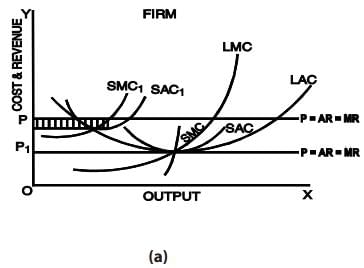
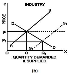
Fig. 21: Long run equilibrium of the firm in a perfectly competitive market
The condition for the long run equilibrium of the firm is that the marginal cost should be equal to the price and the long run average cost i.e. LMC = LAC = P.
The firm adjusts its plant size so as to produce that level of output at which the LAC is the minimum possible. At equilibrium, the short run marginal cost is equal to the long run marginal cost and the short run average cost is equal to the long run average cost. Thus, in the long run we have,
SMC = LMC = SAC = LAC = P = MR
This implies that at the minimum point of the LAC, the corresponding (short run) plant is worked at its optimal capacity, so that the minima of the LAC and SAC coincide. On the other hand, the LMC cuts the LAC at its minimum point and the SMC cuts the SAC at its minimum point. Thus, at the minimum point of the LAC the above equality is achieved.
Long Run Equilibrium of the Industry
A long-run competitive equilibrium of a perfectly competitive industry occurs when three conditions hold:
All firms in the industry are in equilibrium i.e. all firms are maximizing profit.
No firm has an incentive either to enter or exit the industry because all firms are earning zero economic profit or normal profit.
The price of the product is such that the quantity supplied by the industry is equal to the quantity demanded by consumers.
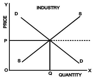
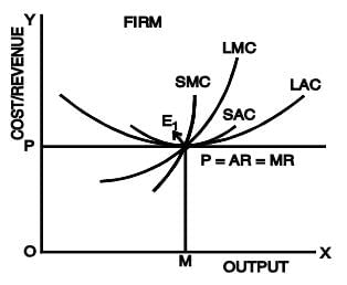
Fig. 22: Long run equilibrium of a competitive industry and its firms
Figure 22 shows that in the long-run AR = MR = LAC = LMC at E1 . In the long run, each firm attains the plant size and output level at which its cost per unit is as low as possible. Since E1 is the minimum point of LAC curve, the firm produces equilibrium output OM at the minimum (optimum) cost. A firm producing output at optimum cost is called an optimum firm. In the long run, all firms under perfect competition are optimum firms having optimum size and these firms charge minimum possible price which just covers their marginal cost.
Thus, in the long run, under perfect competition, the market mechanism leads to optimal allocation of resources. The optimality is shown by the following outcomes associated with the long run equilibrium of the industry:
(a) The output is produced at the minimum feasible cost.
(b) Consumers pay the minimum possible price which just covers the marginal cost i.e. MC = AR. (P = MC)
(c) Plants are used to full capacity in the long run, so that there is no wastage of resources i.e. MC = AC.
(d) Firms earn only normal profits i.e. AC = AR.
(e) Firms maximize profits (i.e. MC = MR), but the level of profits will be just normal.
(f) There is optimum number of firms in the industry.
In other words, in the long run,
LAR = LMR = P = LMC = LAC and there will be optimum allocation of resources.
It should be remembered that the perfectly competitive market system is a myth. This is because the assumptions on which this system is based are never found in the real world market conditions.
|
124 videos|191 docs|88 tests
|
FAQs on Perfect Competition- 2 - Business Economics for CA Foundation
| 1. What is perfect competition in the context of CA Foundation? |  |
| 2. What are the characteristics of perfect competition in CA Foundation? | |
| 3. How does perfect competition determine the market price? | |
| 4. What is producer surplus in perfect competition? | |
| 5. How does perfect competition benefit consumers in CA Foundation? | |

|
4.78/5 Rating |

|
Dec 23, 2024 Last updated |
|
124 videos|191 docs|88 tests
|

|
Explore Courses for CA Foundation exam
|
|
Previous Year Questions with Solutions
,Perfect Competition- 2 | Business Economics for CA Foundation
,video lectures
,past year papers
,Perfect Competition- 2 | Business Economics for CA Foundation
,ppt
,Perfect Competition- 2 | Business Economics for CA Foundation
,Extra Questions
,Viva Questions
,study material
,Objective type Questions
,Sample Paper
,shortcuts and tricks
,Semester Notes
,Summary
,mock tests for examination
,Free
,MCQs
,Exam
,Important questions
,practice quizzes
;


Perfect Competition- 2 Free PDF Download
Importance of Perfect Competition- 2
Perfect Competition- 2 Notes
Perfect Competition- 2 CA Foundation Questions
Study Perfect Competition- 2 on the App
|
© EduRev
|
Education Revolution
|


|


