ICAI Notes- Measures of Central Tendency and Dispersion- 1 | Elementary Mathematics for CDS PDF Download

DEFINITION OF CENTRAL TENDENCY
In many a case, like the distributions of height, weight, marks, profit, wage and so on, it has been noted that starting with rather low frequency, the class frequency gradually increases till it reaches its maximum somewhere near the central part of the distribution and after which the class frequency steadily falls to its minimum value towards the end. Thus, central tendency may be defined as the tendency of a given set of observations to cluster around a single central or middle value and the single value that represents the given set of observations is described as a measure of central tendency or, location, or average. Hence, it is possible to condense a vast mass of data by a single representative value. The computation of a measure of central tendency plays a very important part in many a sphere. A company is recognized by its high average profit, an educational institution is judged on the basis of average marks obtained by its students and so on. Furthermore, the central tendency also facilitates us in providing a basis for comparison between different distribution. Following are the different measures of central tendency:
(i) Arithmetic Mean (AM)
(ii) Median (Me)
(iii) Mode (Mo)
(iv) Geometric Mean(GM)
(v) Harmonic Mean (HM)
CRITERIA FOR AN IDEAL MEASURE OF CENTRAL TENDENCY
Following are the criteria for an ideal measure of central tendency:
(i) It should be properly and unambiguously defined.
(ii) It should be easy to comprehend.
(iii) It should be simple to compute.
(iv) It should be based on all the observations.
(v) It should have certain desirable mathematical properties.
(vi) It should be least affected by the presence of extreme observations.
ARITHMETIC MEAN
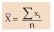
For a given set of observations, the AM may be defined as the sum of all the observations divided by the number of observations. Thus, if a variable x assumes n values x1 , x2 , x3 ,………..xn, then the AM of x, to be denoted by , is given by,
In case of a simple frequency distribution relating to an attribute, we have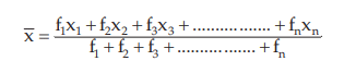
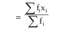
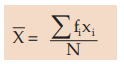
assuming the observation xi occurs fi times, i=1,2,3,……..n and N=≤fi . In case of grouped frequency distribution also we may use formula (15.1.2) with xi as the mid value of the i-th class interval, on the assumption that all the values belonging to the i-th class interval are equal to xi . However, in most cases, if the classification is uniform, we consider the following formula for the computation of AM from grouped frequency distribution: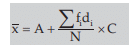
ILLUSTRATIONS:
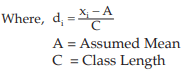
Example : Following are the daily wages in Rupees of a sample of 9 workers: 58, 62, 48, 53, 70, 52, 60, 84, 75. Compute the mean wage.
Solution: Let x denote the daily wage in rupees.
Then as given, x1 =58, x2 =62, x3 = 48, x4 =53, x5 =70, x6 =52, x7 =60, x8 =84 and x9 =75.
Applying the mean wage is given by,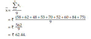
Example : Compute the mean weight of a group of BBA students of St. Xavier’s College from the following data:
Solution: Computation of mean weight of 36 BBA students
Applying, we get the average weight as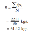
Example 3: Find the AM for the following distribution:
Solution: We apply formula since the amount of computation involved in finding the AM is much more compared to Example Any mid value can be taken as A. However, usually A is taken as the middle most mid-value for an odd number of class intervals and any one of the two middle most mid-values for an even number of class intervals. The class length is taken as C.
Computation of AM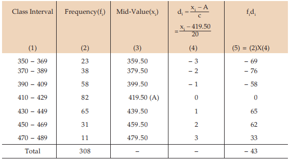
The required AM is given by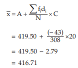
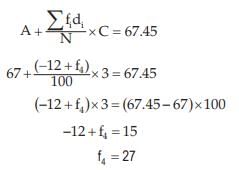
Example : Given that the mean height of a group of students is 67.45 inches. Find the missing frequencies for the following incomplete distribution of height of 100 students.
Solution: Let x denote the height and f3 and f4 as the two missing frequencies.
Estimation of missing frequencies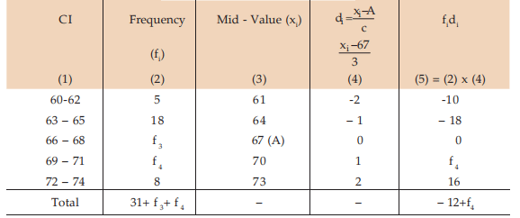
As given, we have ...................(1)
and 
On substituting 27 for f4 in (1), we get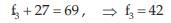
Thus, the missing frequencies would be 42 and 27.
Properties of AM
(i) If all the observations assumed by a variable are constants, say k, then the AM is also k. For example, if the height of every student in a group of 10 students is 170 cm, then the mean height is, of course, 170 cm.
the algebraic sum of deviations of a set of observations from their AM is zero i.e. for unclassified data ,
and for grouped frequency distribution, 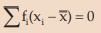 ...............(15.4)
For example, if a variable x assumes five observations, say 58, 63, 37, 45, 29, then . Hence, the deviations of the observations from the AM i.e. )
 are 11.60, 16.60, -9.40,
–1.40 and –17.40, then 11.60 + 16.60 + (–9.40) + (–1.40) + (–17.40) = 0 .
AM is affected due to a change of origin and/or scale which implies that if the original variable x is changed to another variable y by effecting a change of origin, say a, and scale say b, of x i.e. y=a+bx, then the AM of y is given by 
For example, if it is known that two variables x and y are related by 2x+3y+7=0 and , then the AM of y is given by
If there are two groups containing n1 and n2 observations and and
and  as the respective
arithmetic means, then the combined AM is given by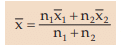
This property could be extended to k>2 groups and we may write
i = 1, 2,........n.
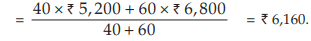
Example : The mean salary for a group of 40 female workers is ₹ 5,200 per month and that for a group of 60 male workers is ₹6800 per month. What is the combined mean salary?
Solution: As given n1 = 40, n2 = 60,  = ₹ 5,200 and
  = ₹ 6,800 hence, the combined mean salary per month is
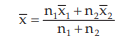
MEDIAN – PARTITION VALUES
As compared to AM, median is a positional average which means that the value of the median is dependent upon the position of the given set of observations for which the median is wanted. Median, for a given set of observations, may be defined as the middle-most value when the observations are arranged either in an ascending order or a descending order of magnitude.
As for example, if the marks of the 7 students are 72, 85, 56, 80, 65, 52 and 68, then in order to find the median mark, we arrange these observations in the following ascending order of magnitude: 52, 56, 65, 68, 72, 80, 85.
Since the 4th term i.e. 68 in this new arrangement is the middle most value, the median mark is 68 i.e. Median (Me) = 68.
As a second example, if the wages of 8 workers, expressed in rupees are
56, 82, 96, 120, 110, 82, 106, 100 then arranging the wages as before, in an ascending order of magnitude, we get ₹ 56, ₹ 82, ₹ 82, ₹ 96, ₹ 100, ₹ 106, ₹ 110, ₹ 120. Since there are two middlemost values, namely, ₹ 96, and ₹100 any value between ₹96 and ₹100 may be, theoretically, regarded as median wage. However, to bring uniqueness, we take the arithmetic mean of the two middle-most values, whenever the number of the observations is an even number. Thus, the median wage in this example, would be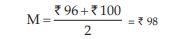
In case of a grouped frequency distribution, we find median from the cumulative frequency distribution of the variable under consideration. We may consider the following formula, which can be derived from the basic definition of median.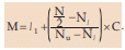
Where,
l1 = lower class boundary of the median class i.e. the class containing median.
N = total frequency.
Nl = less than cumulative frequency corresponding to l1 . (Pre median class)
Nu = less than cumulative frequency corresponding to l2 . (Post median class) l2 being the upper class boundary of the median class. C = l2 – l1 = length of the median class.
Example : Compute the median for the distribution as given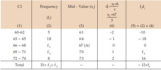
Solution: First, we find the cumulative frequency distribution which is exhibited in Computation of Median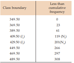
We find, from the Computation of Median  = 154 lies between the two cumulative frequencies 119 and 201 i.e. 119 < 154 < 201 . Thus, we have Nl = 119, Nu = 201 l 1 = 409.50 and l 2 = 429.50. Hence C = 429.50 – 409.50 =20.
Substituting these values in (15.1.7), we get,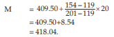
Example : Find the missing frequency from the following data, given that the median mark is 23.
Solution: Let us denote the missing frequency by f3. Table 15.1.5 shows the relevant computation.
(Estimation of missing frequency)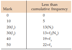
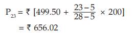
Going through the mark column, we find that 20<23<30. Hence l 1 =20, l 2 =30 and accordingly Nl =13, Nu=13+f3 . Also the total frequency i.e. N is 22+f3 . Thus,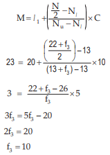
So, the missing frequency is 10.
Properties of median
We cannot treat median mathematically, the way we can do with arithmetic mean. We consider below two important features of median.
(i) If x and y are two variables, to be related by y=a+bx for any two constants a and b, then the median of y is given by
yme = a + bxme
For example, if the relationship between x and y is given by 2x – 5y = 10 and if xme i.e. the median of x is known to be 16.
Then 2x – 5y = 10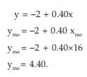
(ii) For a set of observations, the sum of absolute deviations is minimum when the deviations are taken from the median. This property states that | is minimum if we choose A as the median.
PARTITION VALUES OR QUARTILES OR FRACTILES
These may be defined as values dividing a given set of observations into a number of equal parts. When we want to divide the given set of observations into two equal parts, we consider median. Similarly, quartiles are values dividing a given set of observations into four equal parts. So there are three quartiles – first quartile or lower quartile denoted by Q1 , second quartile or median to be denoted by Q2 or Me and third quartile or upper quartile denoted by Q3 . First quartile is the value for which one fourth of the observations are less than or equal to Q1 and the remaining three – fourths observations are more than or equal to Q1 . In a similar manner, we may define Q2 and Q3 .
Deciles are the values dividing a given set of observation into ten equal parts. Thus, there are nine deciles to be denoted by D1 , D2 , D3 ,…..D9 . D1 is the value for which one-tenth of the given observations are less than or equal to D1 and the remaining nine-tenth observations are greater than or equal to D1 when the observations are arranged in an ascending order of magnitude.
Lastly, we talk about the percentiles or centiles that divide a given set of observations into 100 equal parts. The points of sub-divisions being P1 , P2 ,………..P99. P1 is the value for which one hundredth of the observations are less than or equal to P1 and the remaining ninety-nine hundredths observations are greater than or equal to P1 once the observations are arranged in an ascending order of magnitude.
For unclassified data, the pth quartile is given by the (n+1)pth value, where n denotes the total number of observations. p = 1/4, 2/4, 3/4 for Q1, Q2 and Q3 respectively. p=1/10, 2/10,………….9/10. For D1 , D2 ,……,D9 respectively and lastly p=1/100, 2/100,….,99/100 for P1 , P2 , P3 ….P99 respectively.
In case of a grouped frequency distribution, we consider the following formula for the computation of quartiles.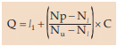
The symbols, except p, have their usual interpretation which we have already discussed while computing median and just like the unclassified data, we assign different values to p depending on the quartile.
Another way to find quartiles for a grouped frequency distribution is to draw the ogive (less than type) for the given distribution. In order to find a particular quartile, we draw a line parallel to the horizontal axis through the point Np. We draw perpendicular from the point of intersection of this parallel line and the ogive. The x-value of this perpendicular line gives us the value of the quartile under discussion.
Example : Following are the wages of the labourers: ₹ 82, ₹56, ₹ 90, ₹ 50, ₹ 120, ₹75, ₹ 75, ₹ 80, ₹130, ₹ 65. Find Q1 , D6 and P82
Solution: Arranging the wages in an ascending order, we get ₹50, ₹56, ₹65, ₹75, ₹75, `₹80, ₹82, ₹90, ₹120, ₹130.
Hence, we have  th value
 th value
= 2.75th value
= 2nd value + 0.75 × difference between the third and the 2nd values.
= ₹56 + 0.75 × (65 – 56)
= ₹62.75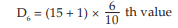
= 6.60th value
= 6th value + 0.60 × difference between the 7th and the 6th values.
= ₹(80 + 0.60 × 2)
= ₹ 81.20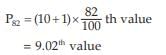
= 9th value + 0.02 × difference between the 10th and the 9th values
= ₹ (120 + 0.02 ×10)
= ₹120.20
Next, let us consider one problem relating to the grouped frequency distribution.
Example : Following distribution relates to the distribution of monthly wages of 100 workers.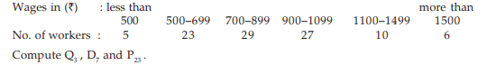
Solution: This is a typical example of an open end unequal classification as we find the lower class limit of the first class interval and the upper class limit of the last class interval are not stated, and theoretically, they can assume any value between 0 and 500 and 1500 to any number respectively. The ideal measure of the central tendency in such a situation is median as the median or second quartile is based on the fifty percent central values. Denoting the first LCB and the last UCB by the L and U respectively, we construct the following cumulative frequency distribution:
Computation of quartiles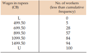
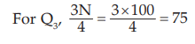
since, 57<75 <84, we take Nl = 57, Nu=84, l1 =899.50, l2 =1099.50, c = l2 –l1 = 200 in the formula for computing Q3 .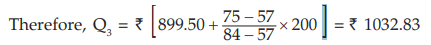
Similarly, for D7 ,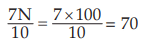 which also lies between 57 and 84.
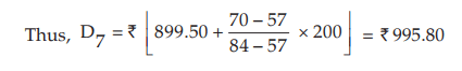

MODE
For a given set of observations, mode may be defined as the value that occurs the maximum number of times. Thus, mode is that value which has the maximum concentration of the observations around it. This can also be described as the most common value with which, even, a layman may be familiar with. Thus, if the observations are 5, 3, 8, 9, 5 and 6, then Mode (Mo) = 5 as it occurs twice and all the other observations occur just once. The definition for mode also leaves scope for more than one mode. Thus sometimes we may come across a distribution having more than one mode. Such a distribution is known as a multi-modal distribution. Bi-modal distribution is one having two modes. Furthermore, it also appears from the definition that mode is not always defined. As an example, if the marks of 5 students are 50, 60, 35, 40, 56, there is no modal mark as all the observations occur once i.e. the same number of times. We may consider the following formula for computing mode from a grouped frequency distribution: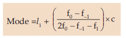
where, l1 = LCB of the modal class. i.e. the class containing mode.
f0 = frequency of the modal class
f–1 = frequency of the pre-modal class
f1 = frequency of the post modal class
C = class length of the modal class
Example : Compute mode for the distribution as described in Example.
Solution: The frequency distribution is shown below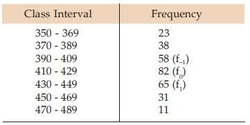
Going through the frequency column, we note that the highest frequency i.e. f0 is 82. Hence, f–1 = 58 and f1 = 65. Also the modal class i.e. the class against the highest frequency is 410 – 429.
Thus l1 = LCB=409.50 and c=429.50 – 409.50 = 20
Hence, applying formulas, we get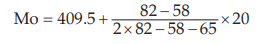
= 421.21 which belongs to the modal class. (410 – 429)
When it is difficult to compute mode from a grouped frequency distribution, we may consider the following empirical relationship between mean, median and mode:
Mean – Mode = 3(Mean – Median)
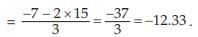
= 3 × 52.40 – 2 × 55.60
= 46.
Example : If y = 2 + 1.50x and mode of x is 15, what is the mode of y?
Solution: By virtue of (11.10), we have
ymo = 2 + 1.50 × 15
= 24.50.
GEOMETRIC MEAN AND HARMONIC MEAN
For a given set of n positive observations, the geometric mean is defined as the n-th root of the product of the observations. Thus if a variable x assumes n values x1 , x2 , x3 ,……….., xn, all the values being positive, then the GM of x is given by
G= (x1 × x2 × x3 ……….. × xn)1/n
For a grouped frequency distribution, the GM is given by
G= (x1 f1 × x2 f2 × x3 f3 …………….. × xn fn )1/N
Where N =
In connection with GM, we may note the following properties :
(i) Logarithm of G for a set of observations is the AM of the logarithm of the observations; i.e.
log G
(ii) if all the observations assumed by a variable are constants, say K > 0, then the GM of the observations is also K.
(iii) GM of the product of two variables is the product of their GM‘s i.e. if z = xy, then GM of z = (GM of x) × (GM of y)
(iv) GM of the ratio of two variables is the ratio of the GM’s of the two variables i.e. if z = x/y then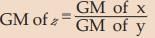
Example : Find the GM of 3, 6 and 12.
Solution: As given x1 =3, x2 =6, x3 =12 and n=3.
Applying , we have G= (3×6×12) 1/3 = (63 )1/3=6.
Example : Find the GM for the following distribution: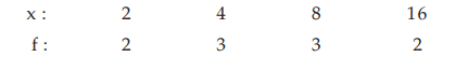
Solution: According to (15.1.12), the GM is given by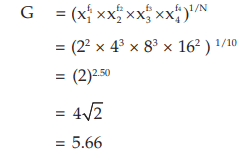
Harmonic Mean
For a given set of non-zero observations, harmonic mean is defined as the reciprocal of the AM of the reciprocals of the observation. So, if a variable x assumes n non-zero values x1 , x2, x3 ,……………,xn, then the HM of x is given by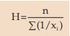
For a grouped frequency distribution, we have
Properties of HM
(i) If all the observations taken by a variable are constants, say k, then the HM of the observations is also k.
(ii) If there are two groups with n1 and n2 observations and H1 and H2 as respective HM’s than the combined HM is given by
Example : Find the HM for 4, 6 and 10.
Solution: Applying (15.1.16), we have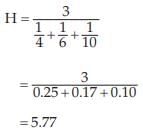
Example : Find the HM for the following data: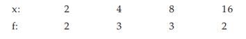
Solution: Using , we get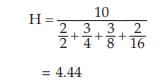
Relation between AM, GM, and HM
For any set of positive observations, we have the following inequality:
AM ≥GM ≥HM
The equality sign occurs, as we have already seen, when all the observations are equal.
Example : compute AM, GM, and HM for the numbers 6, 8, 12, 36.
Solution : In accordance with the definition, we have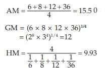
The computed values of AM, GM, and HM establish
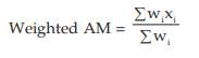
Weighted average
When the observations under consideration have a hierarchical order of importance, we take recourse to computing weighted average, which could be either weighted AM or weighted GM or weighted HM.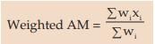
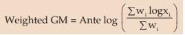
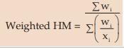
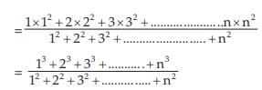
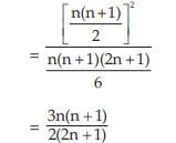
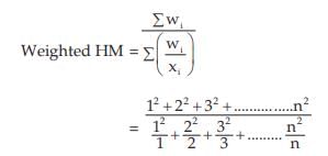
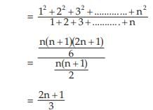
Example : Find the weighted AM and weighted HM of first n natural numbers, the weights being equal to the squares of the corresponding numbers.
Solution: As given,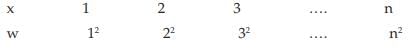
A General review of the different measures of central tendency After discussing the different measures of central tendency, now we are in a position to have a review of these measures of central tendency so far as the relative merits and demerits are concerned on the basis of the requisites of an ideal measure of central tendency which we have already mentioned in section 15.1.2. The best measure of central tendency, usually, is the AM. It is rigidly defined, based on all the observations, easy to comprehend, simple to calculate and amenable to mathematical properties. However, AM has one drawback in the sense that it is very much affected by sampling fluctuations. In case of frequency distribution, mean cannot be advocated for open-end classification. Like AM, median is also rigidly defined and easy to comprehend and compute. But median is not based on all the observation and does not allow itself to mathematical treatment. However, median is not much affected by sampling fluctuation and it is the most appropriate measure of central tendency for an open-end classification. Although mode is the most popular measure of central tendency, there are cases when mo Although mode is the most popular measure of central tendency, there are cases when mode remains undefined. Unlike mean, it has no mathematical property. Mode is also affected by sampling fluctuations. GM and HM, like AM, possess some mathematical properties. They are rigidly defined and based on all the observations. But they are difficult to comprehend and compute and, as such, have limited applications for the computation of average rates and ratios and such like things. |
Example : Given two positive numbers a and b, prove that AH=G2. Does the result hold
for any set of observations?
Solution: For two positive numbers a and b, we have,
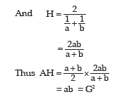
This result holds for only two positive observations and not for any set of observations.
Example : The AM and GM for two observations are 5 and 4 respectively. Find the two
observations.
Solution: If a and b are two positive observations then as given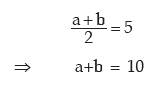
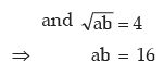
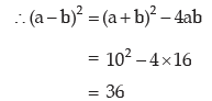
 a – b = 6 (ignoring the negative sign)
Adding (1) and (3) We get,
2a = 16 a = 8
a = 8
From (1), we get b = 10 – a = 2
Thus, the two observations are 8 and 2.
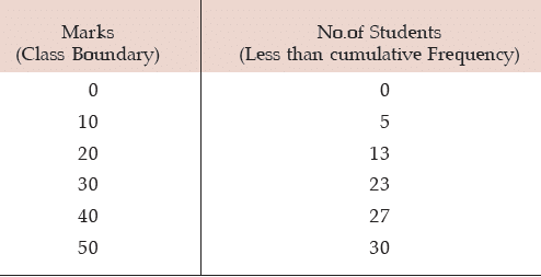
Example : Find the mean and median from the following data:
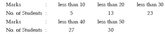
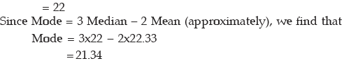
Also compute the mode using the approximate relationship between mean, median and mode.
Solution: What we are given in this problem is less than cumulative frequency distribution.We need to convert this cumulative frequency distribution to the corresponding frequency distribution and thereby compute the mean and median.
Computation of Mean Marks for 30 students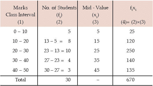
Hence the mean mark is given by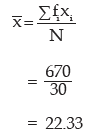
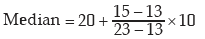
Computation of Median Marks
Since  lies between 13 and 23,
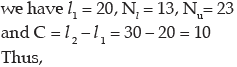
Example : Following are the salaries of 20 workers of a firm expressed in thousand
rupees: 5, 17, 12, 23, 7, 15, 4, 18, 10, 6, 15, 9, 8, 13, 12, 2, 12, 3, 15, 14. The firm gave bonus
amounting to ₹2,000, ₹3,000, ₹ 4,000, ₹5,000 and ₹6,000 to the workers belonging to the salary groups 1,000 – 5,000, 6,000 – 10,000 and so on and lastly 21,000 – 25,000. Find the average bonus paid per employee.
Solution: We first construct frequency distribution of salaries paid to the 20 employees. The average bonus paid per employee is given by Where x i represents the amount of bonus paid to the ith salary group and fi, the number of employees belonging to that group which would be obtained on the basis of frequency distribution of salaries.
Computation of Average bonus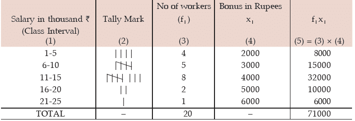
Hence, the average bonus paid per employee

|
174 videos|104 docs|134 tests
|
FAQs on ICAI Notes- Measures of Central Tendency and Dispersion- 1 - Elementary Mathematics for CDS
| 1. What are measures of central tendency? |  |
| 2. How do you calculate the mean? | |
| 3. What is the median and how is it calculated? | |
| 4. How is the mode determined? | |
| 5. What is the purpose of measures of dispersion? | |


practice quizzes
,ICAI Notes- Measures of Central Tendency and Dispersion- 1 | Elementary Mathematics for CDS
,past year papers
,Semester Notes
,study material
,ICAI Notes- Measures of Central Tendency and Dispersion- 1 | Elementary Mathematics for CDS
,Important questions
,Previous Year Questions with Solutions
,Exam
,ICAI Notes- Measures of Central Tendency and Dispersion- 1 | Elementary Mathematics for CDS
,Sample Paper
,Summary
,Viva Questions
,ppt
,Extra Questions
,Objective type Questions
,video lectures
,mock tests for examination
,Free
,MCQs
,shortcuts and tricks
;


ICAI Notes- Measures of Central Tendency and Dispersion- 1 Free PDF Download
Importance of ICAI Notes- Measures of Central Tendency and Dispersion- 1
ICAI Notes- Measures of Central Tendency and Dispersion- 1
ICAI Notes- Measures of Central Tendency and Dispersion- 1 CDS Questions
Study ICAI Notes- Measures of Central Tendency and Dispersion- 1 on the App
|
© EduRev
|
Education Revolution
|


|


