ICAI Notes: Probability- 1 | Quantitative Aptitude for CA Foundation PDF Download
INTRODUCTION
The terms 'Probably' 'in all likelihood', 'chance', 'odds in favour', 'odds against' are too familiar nowadays and they have their origin in a branch of Mathematics, known as Probability. In recent time, probability has developed itself into a full-fledged subject and become an integral part of statistics. The theories of Testing Hypothesis and Estimation are based on probability.
It is rather surprising to know that the first application of probability was made by a group of mathematicians in Europe about three hundreds years back to enhance their chances of
winning in different games of gambling. Later on, the theory of probability was developed by Abraham De Moicere and Piere-Simon De Laplace of France, Reverend Thomas Bayes and R.
A. Fisher of England, Chebyshev, Morkov, Khinchin, Kolmogorov of Russia and many other noted mathematicians as well as statisticians.
Two broad divisions of probability are Subjective Probability and Objective Probability.
Subjective Probability is basically dependent on personal judgement and experience and, as such, it may be influenced by the personal belief, attitude and bias of the person applying it.
However in the field of uncertainty, this would be quite helpful and it is being applied in the area of decision making management. This Subjective Probability is beyond the scope of our present discussion. We are going to discuss Objective Probability in the remaining sections.
RANDOM EXPERIMENT
In order to develop a sound knowledge about probability, it is necessary to get ourselves familiar with a few terms.
Experiment: An experiment may be described as a performance that produces certain results.
Random Experiment: An experiment is defined to be random if the results of the experiment depend on chance only. For example if a coin is tossed, then we get two outcomes—Head (H) and Tail (T). It is impossible to say in advance whether a Head or a Tail would turn up when we toss the coin once. Thus, tossing a coin is an example of a random experiment. Similarly, rolling a dice (or any number of dice), drawing items from a box containing both defective and non—defective items, drawing cards from a pack of well shuffled fifty—two cards etc. are all random experiments.
Events: The results or outcomes of a random experiment are known as events. Sometimes
events may be combination of outcomes. The events are of two types:
(i) Simple or Elementary,
(ii) Composite or Compound.
An event is known to be simple if it cannot be decomposed into further events. Tossing a coin once provides us two simple events namely Head and Tail. On the other hand, a composite event is one that can be decomposed into two or more events. Getting a head when a coin is tossed twice is an example of composite event as it can be split into the events HT and TH which are both elementary events.
Mutually Exclusive Events or Incompatible Events: A set of events A1, A2, A3, …… is known to be mutually exclusive if not more than one of them can occur simultaneously. Thus occurrence of one such event implies the non-occurrence of the other events of the set. Once a coin is tossed, we get two mutually exclusive events Head and Tail.
Exhaustive Events: The events A1, A2, A3, ………… are known to form an exhaustive set if one of these events must necessarily occur. As an example, the two events Head and Tail,
when a coin is tossed once, are exhaustive as no other event except these two can occur.
Equally Likely Events or Mutually Symmetric Events or Equi-Probable Events: The events of a random experiment are known to be equally likely when all necessary evidence are taken into account, no event is expected to occur more frequently as compared to the other events of the set of events. The two events Head and Tail when a coin is tossed is an example of a pair of equally likely events because there is no reason to assume that Head (or Tail) would occur more frequently as compared to Tail (or Head).
CLASSICAL DEFINITION OF PROBABILITY OR A PRIOR DEFINITION
Let us consider a random experiment that result in n finite elementary events, which are
assumed to be equally likely. We next assume that out of these n events, nA ( ≤n) events are favourable to an event A. Then the probability of occurrence of the event A is defined as the ratio of the number of events favourable to A to the total number of events. Denoting this by P(A), we have ............(1)
However if instead of considering all elementary events, we focus our attention to only those composite events, which are mutually exclusive, exhaustive and equally likely and if m( ≤ n) denotes such events and is furthermore mA( ≤nA) denotes the no. of mutually exclusive, exhaustive and equally likely events favourable to A, then we have
For this definition of probability, we are indebted to Bernoulli and Laplace. This definition is also termed as a priori definition because probability of the event A is defined on the basis of prior knowledge.
This classical definition of probability has the following demerits or limitations:
(i) It is applicable only when the total no. of events is finite.
(ii) It can be used only when the events are equally likely or equi-probable. This assumption is made well before the experiment is performed.
(iii) This definition has only a limited field of application like coin tossing, dice throwing,
drawing cards etc. where the possible events are known well in advance. In the field of
uncertainty or where no prior knowledge is provided, this definition is inapplicable.
In connection with classical definition of probability, we may note the following points:
(a) The probability of an event lies between 0 and 1, both inclusive. i.e. 0≤P(A) ≤ 1 When P(A) = 0, A is known to be an impossible event and when P(A) = 1, A is known to be a sure event. in favour of the event A and its inverse ratio is known as odds against the event A. i.e. odds in favour of A = mA : (m – mA) and odds against A = (m – mA) : mA |
 and it is known as complimentary event of A. The event A along with its complimentary A’ forms a set of mutually exclusive and exhaustive events.
ILLUSTRATIONS:
Example: A coin is tossed three times. What is the probability of getting:
(i) 2 heads
(ii) at least 2 heads
Solution: When a coin is tossed three times, first we need enumerate all the elementary events. This can be done using 'Tree diagram' as shown below: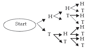
Hence the elementary events are
HHH, HHT, HTH, HTT, THH, THT, TTH, TTT
Thus the number of elementary events (n) is 8.
(i) Out of these 8 outcomes, 2 heads occur in three cases namely HHT, HTH and THH. If we denote the occurrence of 2 heads by the event A and if assume that the coin as well as
performer of the experiment is unbiased then this assumption ensures that all the eight
elementary events are equally likely. Then by the classical definition of probability, we
have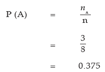
(ii) Let B denote occurrence of at least 2 heads i.e. 2 heads or 3 heads. Since 2 heads occur in 3 cases and 3 heads occur in only 1 case, B occurs in 3 + 1 or 4 cases. By the classical
definition of probability,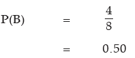
Example: A dice is rolled twice. What is the probability of getting a difference of 2 points?
Solution: If an experiment results in p outcomes and if the experiment is repeated q times, then the total number of outcomes is pq. In the present case, since a dice results in 6 outcomes and the dice is rolled twice, total no. of outcomes or elementary events is 62 or 36. We assume that the dice is unbiased which ensures that all these 36 elementary events are equally likely. Now a difference of 2 points in the uppermost faces of the dice thrown twice can occur in the following cases:
Thus denoting the event of getting a difference of 2 points by A, we find that the no. of
outcomes favourable to A, from the above table, is 8. By classical definition of probability, we get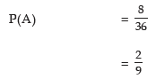
Example: Two dice are thrown simultaneously. Find the probability that the sum of
points on the two dice would be 7 or more.
Solution: If two dice are thrown then, as explained in the last problem, total no. of elementary events is 62 or 36. Now a total of 7 or more i.e. 7 or 8 or 9 or 10 or 11 or 12 can occur only in the following combinations: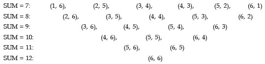
Thus the no. of favourable outcomes is 21. Letting A stand for getting a total of 7 points or
more, we have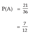
Example: What is the chance of picking a spade or an ace not of spade from a pack of 52 cards?
Solution: A pack of 52 cards contain 13 Spades, 13 Hearts, 13 Clubs and 13 Diamonds. Each of these groups of 13 cards has an ace. Hence the total number of elementary events is 52 out of which 13 + 3 or 16 are favourable to the event A representing picking a Spade or an ace not of Spade. Thus we have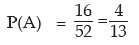
Example: Find the probability that a four digit number comprising the digits 2, 5, 6 and
7 would be divisible by 4.
Solution: Since there are four digits, all distinct, the total number of four digit numbers that can be formed without any restriction is 4! or 4 × 3 × 2 × 1 or 24. Now a four digit number would be divisible by 4 if the number formed by the last two digits is divisible by 4. This could happen when the four digit number ends with 52 or 56 or 72 or 76. If we fix the last two digits by 52, and then the 1st two places of the four digit number can be filled up using the remaining 2 digits in 2! or 2 ways. Thus there are 2 four digit numbers that end with 52. Proceeding in this manner, we find that the number of four digit numbers that are divisible by 4 is 4 × 2 or 8. If (A) denotes the event that any four digit number using the given digits would be divisible by 4, then we have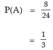
Example: A committee of 7 members is to be formed from a group comprising 8 gentlemen and 5 ladies. What is the probability that the committee would comprise:
(a) 2 ladies,
(b) at least 2 ladies.
Solution: Since there are altogether 8 + 5 or 13 persons, a committee comprising 7 members can be formed in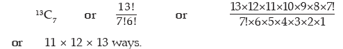
(a) When the committee is formed taking 2 ladies out of 5 ladies, the remaining (7–2) or 5
committee members are to be selected from 8 gentlemen. Now 2 out of 5 ladies can be
selected in 5C2 ways and 5 out of 8 gentlemen can be selected in 8C5 ways. Thus if A
denotes the event of having the committee with 2 ladies, then A can occur in 5C2× 8C5 or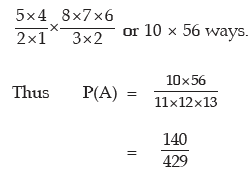
(b) Since the minimum number of ladies is 2, we can have the following combinations: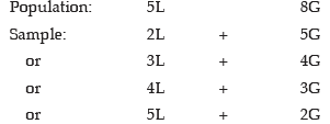
Thus if B denotes the event of having at least two ladies in the committee, then B can occur in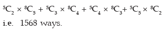
Hence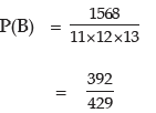
RELATIVE FREQUENCY DEFINITION OF PROBABILITY
Owing to the limitations of the classical definition of probability, there are cases when we
consider the statistical definition of probability based on the concept of relative frequency.
This definition of probability was first developed by the British mathematicians in connection with the survival probability of a group of people.
Let us consider a random experiment repeated a very good number of times, say n, under an identical set of conditions. We next assume that an event A occurs fA times. Then the limiting value of the ratio of fA to n as n tends to infinity is defined as the probability of A.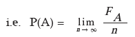
This statistical definition is applicable if the above limit exists and tends to a finite value.
Example 16.7: The following data relate to the distribution of wages of a group of workers:
If a worker is selected at random from the entire group of workers, what is the probability that
(a) his wage would be less than ₹ 50?
(b) his wage would be less than ₹ 80?
(c) his wage would be more than ₹ 100?
(d) his wages would be between ₹ 70 and ₹ 100?
Solution: As there are altogether 150 workers, n = 150.
(a) Since there is no worker with wage less than ₹ 50, the probability that the wage of a
randomly selected worker would be less than ₹ 50 is P(A)= 
(b) Since there are (15+23+36) or 74 worker having wages less than ₹80 out of a group of
150 workers, the probability that the wage of a worker, selected at random from the
group, would be less than ₹80 is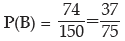
(c) There are (12+5) or 17 workers with wages more than ₹ 100. Thus the probability of finding a worker, selected at random, with wage more than ₹ 100 is 
(d) There are (36+42+17) or 95 workers with wages in between ₹ 70 and ₹100. Thus
OPERATIONS ON EVENTS-SET THEORETIC APPROACH TO PROBABILITY
Applying the concept of set theory, we can give a new dimension of the classical definition of probability. A sample space may be defined as a non-empty set containing all the elementary events of a random experiment as sample points. A sample space is denoted by S or Ω . An event A may be defined as a non-empty subset of S. This is shown in Figure 16.1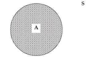
Showing an event A  and the sample space S
As for example, if a dice is rolled once than the sample space is given by
S = {1, 2, 3, 4, 5, 6}.
Next, if we define the events A, B and C such that
A = {x: x is an even no. of points in S}
B = {x: x is an odd no. of points in S}
C = {x: x is a multiple of 3 points in S}
Then, it is quite obvious that
A = {2, 4, 6}, B = {1, 3, 5} and C = {3, 6}.
The classical definition of probability may be defined in the following way.
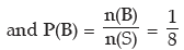
Let us consider a finite sample space S i.e. a sample space with a finite no. of sample points, n (S). We assume that all these sample points are equally likely. If an event A which is a subset of S, contains n (A) sample points, then the probability of A is defined as the ratio of the number of sample points in A to the total number of sample points in S. i.e.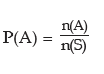
Union of two events A and B is defined as a set of events containing all the sample points of event A or event B or both the events. This is shown in Figure 17.2 we have A∩ B = {x:x∈A on x∈ B}.
where x denotes the sample points.
Showing the union of two events A and B and also their intersection
In the above example, we have A∪C = {2, 3, 4, 6} and A∪B = {1, 2, 3, 4, 5, 6}.
The intersection of two events A and B may be defined as the set containing all the sample
points that are common to both the events A and B. This is shown in Figure 16.2. we have
A∩B = {x:x∈A and x ∈B }.
In the above example, A ∩ B = ϕ
A ∩ C = {6}
Since the intersection of the events A and B is a null set ϕ , it is obvious that A and B are
mutually exclusive events as they cannot occur simultaneously.
The difference of two events A and B, to be denoted by A – B, may be defined as the set of
sample points present in set A but not in B. i.e.
A – B = {x:x∈A and x ∉ B}.
Similarly, B – A = {x:x∈ B and x∉ A}.
In the above examples,
A – B = ϕ
And A – C = {2, 4}.
This is shown in Figure.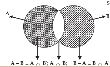
Showing (A – B) and (B – A)
The complement of an event A may be defined as the difference between the sample space S
and the event A. i.e.
A’= {x: x ∈ S and x ∉ A}.
In the above example A’= S – A
= {1, 3, 5}
Figure depicts A’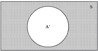
Showing A’
Now we are in a position to redefine some of the terms we have already discussed in section (17.2). Two events A and B are mutually exclusive if P (A ∩ B) = 0 or more precisely,....(16.9)
P (A∪ B) = P(A) + P(B)
Similarly three events A, B and C are mutually exclusive if
P (A∪ B∪ C) = P(A) + P(B) + P(C)
Two events A and B are exhaustive if
P(A ∪ B) = 1
Similarly three events A, B and C are exhaustive if
P(A ∪ B∪ C) = 1
Three events A, B and C are equally likely if
P(A) = P(B) = P(C)
Example: Three events A, B and C are mutually exclusive, exhaustive and equally likely.
What is the probability of the complementary event of A?
Solution: Since A, B and C are mutually exclusive, we have
P(A ∪ B∪ C) = P(A) + P(B) + P(C) …………. (1)
Since they are exhaustive, P(A∪ B∪ C) =1 …………. (2)
Since they are also equally likely, P(A) = P(B) = P(C) = K, Say ………….(3)
Combining equations (1), (2) and (3), we have
1 = K + K + K
⇒ K = 1/3
Thus P(A) = P(B) = P(C) = 1/3
Hence P(A’) = 1 – 1/3 = 2/3
AXIOMATIC OR MODERN DEFINITION OF PROBABILITY
Let us consider a sample space S in connection with a random experiment and let A be an
event defined on the sample space S i.e. A ⊆ S. Then a real valued function P defined on S is known as a probability measure and P(A) is defined as the probability of A if P satisfies the following axioms:
(i) P(A) ≥ 0 for every A ⊆ S (subset) (ii) P(S) = 1 (iii) For any sequence of mutually exclusive events A1, A2, A3,.. P(A1 ∪ A2 ∪ A3 ∪….) = P(A1) + P(A2) + P(A3) + |
ADDITION THEOREMS OR THEOREMS ON TOTAL PROBABILITY
Theorem 1 For any two mutually exclusive events A and B, the probability that either A or B occurs is given by the sum of individual probabilities of A and B.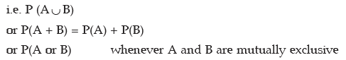
Example: A number is selected from the first 25 natural numbers. What is the probability that it would be divisible by 4 or 7?
Solution: Let A be the event that the number selected would be divisible by 4 and B, the event that the selected number would be divisible by 7. Then AUB denotes the event that the number would be divisible by 4 or 7. Next we note that A = {4, 8, 12, 16, 20, 24} and B = {7, 14, 21} whereas S = {1, 2, 3, ……... 25}. Since A ∩ B = ϕ , the two events A and B are mutually exclusive and as such we have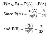
Thus from (1), we have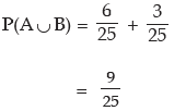
Hence the probability that the selected number would be divisible by 4 or 7 is 9/25 or 0.36
Example 16.10: A coin is tossed thrice. What is the probability of getting 2 or more heads?
Solution: If a coin is tossed three times, then we have the following sample space.
S = {HHH, HHT, HTH, HTT, THH, THT, TTH, TTT} 2 or more heads imply 2 or 3 heads.
If A and B denote the events of occurrence of 2 and 3 heads respectively, then we find that
A = {HHT, HTH, THH} and B = {HHH}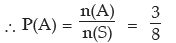
As A and B are mutually exclusive, the probability of getting 2 or more heads is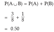
Theorem 2 For any K( ≥ 2) mutually exclusive events A1, A2, A3 …, AK the probability that at least one of them occurs is given by the sum of the individual probabilities of the K events.
Obviously, this is an extension of Theorem 1.
Theorem 3 For any two events A and B, the probability that either A or B occurs is given by
the sum of individual probabilities of A and B less the probability of simultaneous occurrence of the events A and B.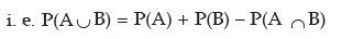
This theorem is stronger than Theorem 1 as we can derive Theorem 1 from Theorem 3 and not Theorem 3 from Theorem 1. For want of sufficient evidence, it is wiser to apply Theorem 3 for evaluating total probability of two events.
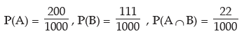
Example: A number is selected at random from the first 1000 natural numbers. What is the probability that it would be a multiple of 5 or 9?
Solution: Let A, B, A ∪ B and A∩ B denote the events that the selected number would be a multiple of 5, 9, 5 or 9 and both 5 and 9 i.e. LCM of 5 and 9 i.e. 45 respectively.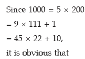
Hence the probability that the selected number would be a multiple of 4 or 9 is given by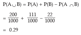
Example: The probability that an Accountant's job applicant has a B. Com. Degree is
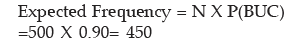
0.85, that he is a CA is 0.30 and that he is both B. Com. and CA is 0.25 out of 500 applicants, how many would be B. Com. or CA?
Solution: Let the event that the applicant is a B. Com. be denoted by B and that he is a CA be denoted by C Then as given,
P(B) = 0.85, P(C) = 0.30 and P(B ∩ C) = 0.25
The probability that an applicant is B. Com. or CA is given by
P(B ∪ C) = P(B) + P(C) – P(B ∩ C)
= 0.85 + 0.30 – 0.25
= 0.90
Expected frequency = N × P (B ∪ C)
Expected frequency = 500 × 9.90 = 450
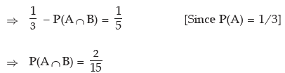
Example: If P(A–B) = 1/5, P(A) = 1/3 and P (B) = 1/2, what is the probability that out
of the two events A and B, only B would occur?
Solution: A glance at Figure 17.3 suggests that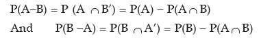
Also (16.21) and (16.22) describe the probabilities of occurrence of the event only A and only B respectively.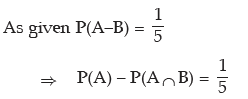
The probability that the event B only would occur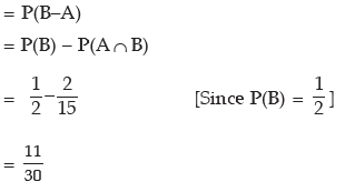
Theorem 4 For any three events A, B and C, the probability that at least one of the events
occurs is given by
P(A ∪ B∪ C) = P(A) + P(B) + P(C) – P(A ∩ B) – P(A ∩ C) – P(B ∩ C)+ P(A ∩ B∩ C)
Following is an application of this theorem.
Example: There are three persons A, B and C having different ages. The probability that A survives another 5 years is 0.80, B survives another 5 years is 0.60 and C survives another 5 years is 0.50. The probabilities that A and B survive another 5 years is 0.46, B and C survive another 5 years is 0.32 and A and C survive another 5 years 0.48. The probability that all these three persons survive another 5 years is 0.26. Find the probability that at least one of them survives another 5 years.
Solution: As given P(A) = 0.80, P(B) = 0.60, P(C) = 0.50,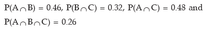
The probability that at least one of them survives another 5 years in given by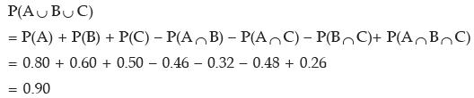
|
148 videos|174 docs|99 tests
|
FAQs on ICAI Notes: Probability- 1 - Quantitative Aptitude for CA Foundation
| 1. What is probability and how is it related to the CA Foundation exam? |  |
| 2. What are the different types of probability? | |
| 3. How can I calculate the probability of independent events? | |
| 4. What is the difference between permutation and combination in probability? | |
| 5. How can I use probability to solve real-life problems? | |

|
1.5K Views |

|
4.73/5 Rating |

|
Nov 23, 2024 Last updated |
|
148 videos|174 docs|99 tests
|

|
Explore Courses for CA Foundation exam
|
|
study material
,MCQs
,Summary
,ICAI Notes: Probability- 1 | Quantitative Aptitude for CA Foundation
,Exam
,video lectures
,mock tests for examination
,ICAI Notes: Probability- 1 | Quantitative Aptitude for CA Foundation
,practice quizzes
,Semester Notes
,Important questions
,Sample Paper
,Free
,Extra Questions
,ICAI Notes: Probability- 1 | Quantitative Aptitude for CA Foundation
,past year papers
,shortcuts and tricks
,Viva Questions
,ppt
,Previous Year Questions with Solutions
,Objective type Questions
,


ICAI Notes: Probability- 1 Free PDF Download
Importance of ICAI Notes: Probability- 1
ICAI Notes: Probability- 1
ICAI Notes: Probability- 1 CA Foundation Questions
Study ICAI Notes: Probability- 1 on the App
|
© EduRev
|
Education Revolution
|


Follow Us
|