ICAI Notes: Theoretical Distribution- 1 | Quantitative Aptitude for CA Foundation PDF Download

INTRODUCTION
In chapter seventeen, it may be recalled, we discussed frequency distribution. In a similar manner, we may think of a probability distribution where just like distributing the total frequency to different class intervals, the total probability (i.e. one) is distributed to different mass points in case of a discrete random variable or to different class intervals in case of a continuous random variable. Such a probability distribution is known as Theoretical Probability Distribution, since such a distribution exists in theory. We need to study theoretical probability distribution for the following important factors:
(a) An observed frequency distribution, in many a case, may be regarded as a sample i.e. a representative part of a large, unknown, boundless universe or population and we may be interested to know the form of such a distribution. By fitting a theoretical probability distribution to an observed frequency distribution of, say, the lamps produced by a manufacturer, it may be possible for the manufacturer to specify the length of life of the lamps produced by him up to a reasonable degree of accuracy. By studying the effect of a particular type of missiles, it may be possible for our scientist to suggest the number of such missiles necessary to destroy an army position. By knowing the distribution of smokers, a social activist may warn the people of a locality about the nuisance of active and passive smoking and so on.
(b) Theoretical probability distribution may be profitably employed to make short term projections for the future.
(c) Statistical analysis is possible only on the basis of theoretical probability distribution. Setting confidence limits or testing statistical hypothesis about population parameter(s) is based on the probability distribution of the population under consideration. A probability distribution also possesses all the characteristics of an observed distribution. We define mean (μ) , median , mode  (μ₀ ) , standard deviation (σ ) etc. exactly same way we have done earlier. Again a probability distribution may be either a discrete probability distribution or a Continuous probability distribution depending on the random variable under study. Two important discrete probability distributions are (a) Binomial Distribution and (b) Poisson distribution. 
Some important continuous probability distributions are Normal Distribution

BINOMIAL DISTRIBUTION
One of the most important and frequently used discrete probability distribution is Binomial Distribution. It is derived from a particular type of random experiment known as Bernoulli process named after the famous mathematician Bernoulli. Noting that a 'trial' is an attempt to produce a particular outcome which is neither certain nor impossible, the characteristics of Bernoulli trials are stated below:
(i) Each trial is associated with two mutually exclusive and exhaustive outcomes, the occurrence of one of which is known as a 'success' and as such its non occurrence as a 'failure'. As an example, when a coin is tossed, usually occurrence of a head is known as a success and its non–occurrence i.e. occurrence of a tail is known as a failure.
(ii) The trials are independent.
(iii) The probability of a success, usually denoted by p, and hence that of a failure, usually denoted by q = 1–p, remain unchanged throughout the process.
(iv) The number of trials is a finite positive integer. A discrete random variable x is defined to follow binomial distribution with parameters n and p, to be denoted by x ~ B (n, p), if the probability mass function of x is given by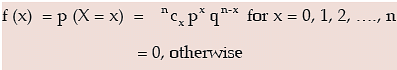

We may note the following important points in connection with binomial distribution: (a) As n >0, p, q ≥ 0, it follows that f(x) ≥ 0 for every x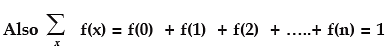

(b) Binomial distribution is known as biparametric distribution as it is characterised by two parameters n and p. This means that if the values of n and p are known, then the distribution is known completely.
(c) The mean of the binomial distribution is given by μ = np
(d) Depending on the values of the two parameters, binomial distribution may be unimodal or bi- modal.μ₀, the mode of binomial distribution, is given by μ₀ = the largest integer contained in (n+1)p if (n+1)p is a non-integer (n+1)p and (n+1)p - 1 if (n+1)p is an integer
(e) The variance of the binomial distribution is given by
Since p and q are numerically less than or equal to 1, npq < np
⇒ variance of a binomial variable is always less than its mean. Also variance of X attains its maximum value at p = q = 0.5 and this maximum value is n/4.
(f) Additive property of binomial distribution. If X and Y are two independent variables such that
X~B (n₁, P)
and Y~B (n₂₁P)
Then (X+Y) ~B (n₁ + n₂ , P)
Applications of Binomial Distribution
Binomial distribution is applicable when the trials are independent and each trial has just two outcomes success and failure. It is applied in coin tossing experiments, sampling inspection plan, genetic experiments and so on.
Example: A coin is tossed 10 times. Assuming the coin to be unbiased, what is the probability of getting
(i) 4 heads?
(ii) at least 4 heads?
(iii) at most 3 heads?
Solution: We apply binomial distribution as the tossing are independent of each other. With every tossing, there are just two outcomes either a head, which we call a success or a tail, which we call a failure and the probability of a success (or failure) remains constant throughout.
Let X denotes the no. of heads. Then X follows binomial distribution with parameter n = 8 and p = 1/2 (since the coin is unbiased). Hence q = 1 – p = 1/2
The probability mass function of X is given by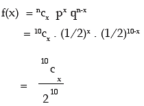


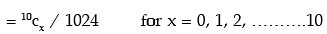
(i) probability of getting 4 heads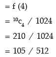

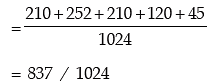
(ii) probability of getting at least 4 heads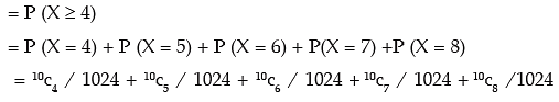


(iii ) probability of getting at most 3 heads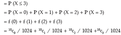


Example: If 15 dates are selected at random, what is the probability of getting two Sundays?
Solution: If X denotes the number at Sundays, then it is obvious that X follows binomial distribution with parameter n = 15 and p = probability of a Sunday in a week = 1/7 and q = 1 – p = 6 / 7.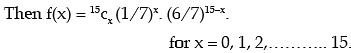

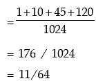
Hence the probability of getting two Sundays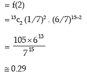

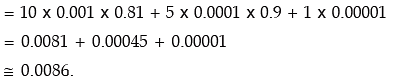
Example: The incidence of occupational disease in an industry is such that the workmen have a 10% chance of suffering from it. What is the probability that out of 5 workmen, 3 or more will contract the disease?
Solution: Let X denote the number of workmen in the sample. X follows binomial with parameters n = 5 and p = probability that a workman suffers from the occupational disease = 0.1
Hence q = 1 – 0.1 = 0.9.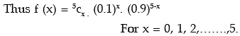

The probability that 3 or more workmen will contract the disease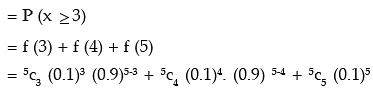

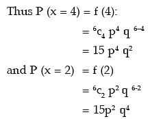
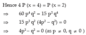
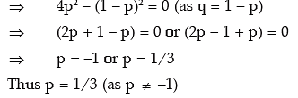
Example: Find the probability of a success for the binomial distribution satisfying the

following relation 4 P (x = 4) = P (x = 2) and having the parameter n as six.

Solution: We are given that n = 6. The probability mass function of x is given by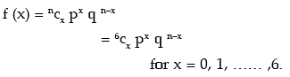

Example: Find the binomial distribution for which mean and standard deviation are 6 and 2 respectively.
Solution: Let x ~ B (n, p)
Given that mean of x = np = 6 … ( 1 )
and SD of x = 2
⇒ variance of x = npq = 4 ….. ( 2 )
Dividing ( 2 ) by ( 1 ), we get q = 2/3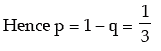

Replacing p by 1/3 in equation ( 1 ), we get
n =18
Thus the probability mass function of x is given by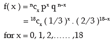

Example: Fit a binomial distribution to the following data: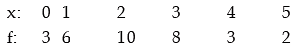

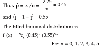
Solution: In order to fit a theoretical probability distribution to an observed frequency distribution it is necessary to estimate the parameters of the probability distribution. There are several methods of estimating population parameters. One rather, convenient method is ‘Method of Moments’. This comprises equating p moments of a probability distribution to p moments of the observed frequency distribution, where p is the number of parameters to be estimated. Since n = 5 is given, we need estimate only one parameter p. We equate the first moment about origin i.e. AM of the probability distribution to the AM of the given distribution and estimate p.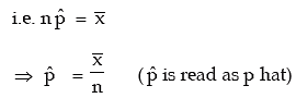

The fitted binomial distribution is then given by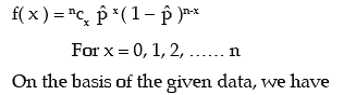




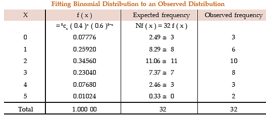
A look at Table  suggests that the fitting of binomial distribution to the given frequency distribution is satisfactory.
Example: 6 coins are tossed 512 times. Find the expected frequencies of heads. Also, compute the mean and SD of the number of heads.
Solution: If x denotes the number of heads, then x follows binomial distribution with parameters n = 6 and p = prob. of a head = ½, assuming the coins to be unbiased. The probability mass function of x is given by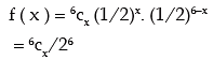

for x = 0, 1, …..6.
The expected frequencies are given by Nf ( x ).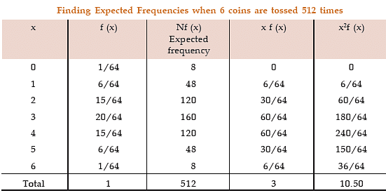



Applying formula for mean and SD,
we get μ = np = 6 x 1/2 = 3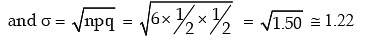

Example: An experiment succeeds thrice as after it fails. If the experiment is repeated 5 times, what is the probability of having no success at all ?
Solution: Denoting the probability of a success and failure by p and q respectively, we have,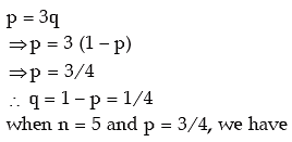


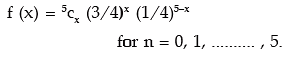
So probability of having no success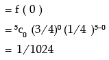

Example: What is the mode of the distribution for which mean and SD are 10 and √5 respectively.
Solution: As given np = 10 .......... (1)

on solving (1) and (2), we get n = 20 and p = 1/2
Hence mode = Largest integer contained in (n+1)p
= Largest integer contained in (20+1) × 1/2
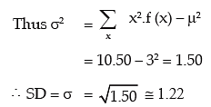
= Largest integer contained in 10.50
= 10.
Example: If x and y are 2 independent binomial variables with parameters 6 and 1/2 and 4 and 1/2 respectively, what is P ( x + y ≥ 1 )?
Solution: Let z = x + y.
It follows that z also follows binomial distribution with parameters
( 6 + 4 ) and 1/2
i.e. 10 and 1/2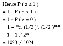


POISSON DISTRIBUTION
Poisson distribution is a theoretical discrete probability distribution which can describe many processes. Simon Denis Poisson of France introduced this distribution way back in the year 1837.
Poisson Model
Let us think of a random experiment under the following conditions:
I. The probability of finding success in a very small time interval ( t, t + dt ) is kt, where k (>0) is a constant.
II. The probability of having more than one success in this time interval is very low.
III. The probability of having success in this time interval is independent of t as well as earlier successes.
The above model is known as Poisson Model. The probability of getting x successes in a relatively long time interval T containing m small time intervals t i.e. T = mt. is given by

for x = 0, 1, 2, ......… ∞
Taking kT = m, the above form is reduced to

for x = 0, 1, 2, ......… ∞

Definition of Poisson Distribution
A random variable X is defined to follow Poisson distribution with parameter λ, to be denoted by X ~ P (m) if the probability mass function of x is given by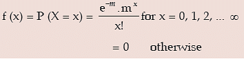

Here e is a transcendental quantity with an approximate value as 2.71828.
It is wiser to remember the following important points in connection with Poisson distribution:
(i) Since e^–m = 1/e^m >0, whatever may be the value of m, m > 0, it follows that f (x) ≥ 0 for every x. Also it can be established that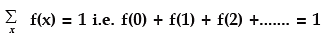
(ii) Poisson distribution is known as a uniparametric distribution as it is characterised by only one parameter m.
(iii) The mean of Poisson distribution is given by m i,e μ = m.
(iv) The variance of Poisson distribution is given by σ² = m
(v) Like binomial distribution, Poisson distribution could be also unimodal or bimodal depending upon the value of the parameter m.
We have μ₀ = The largest integer contained in m if m is a non-integer
= m and m–1 if m is an integer
(vi) Poisson approximation to Binomial distribution If n, the number of independent trials of a binomial distribution, tends to infinity and p, the probability of a success, tends to zero, so that m = np remains finite, then a binomial distribution with parameters n and p can be approximated by a Poisson distribution with parameter m (= np). In other words when n is rather large and p is rather small so that m = np is moderate then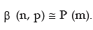
(vii) Additive property of Poisson distribution
If X and y are two independent variables following Poisson distribution with parameters m₁ and m₂ respectively, then Z = X + Y also follows Poisson distribution with parameter (m₁ + m₂ ).
i.e. if X ~ P (m₁) and Y ~ P (m₂) and X and Y are independent, then
Z = X + Y ~ P (m₁ + m₂ )
Application of Poisson distribution
Poisson distribution is applied when the total number of events is pretty large but the probability of occurrence is very small. Thus we can apply Poisson distribution, rather profitably, for the following cases:

Example: Find the mean and standard deviation of x where x is a Poisson variate satisfying the condition P (x = 2) = P ( x = 3).
Solution: Let x be a Poisson variate with parameter m. The probability max function of x is then given by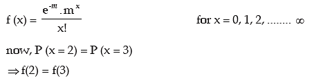



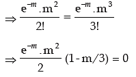
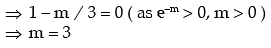
Thus the mean of this distribution is m = 3 and standard deviation = √3 ≌ 1.73
Example: The probability that a random variable x following Poisson distribution would assume a positive value is (1 – e^–2.7). What is the mode of the distribution?
Solution: If x ~ P (m), then its probability mass function is given by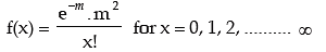

The probability that x assumes a positive value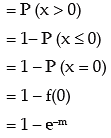

As given,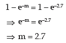

Thus μ₀ = largest integer contained in 2.7
= 2
Example: The standard deviation of a Poisson variate is 1.732. What is the probability that the variate lies between –2.3 to 3.68?
Solution: Let x be a Poisson variate with parameter m.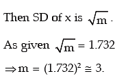

The probability that x lies between –2.3 and 3.68
= P(– 2.3 < x < 3.68)
= f(0) + f(1) + f(2) + f(3)        (As x can assume 0, 1, 2, 3, 4 .....)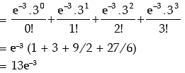

Example: X is a Poisson variate satisfying the following relation:
P (X = 2) = 9P (X = 4) + 90P (X = 6).
What is the standard deviation of X?
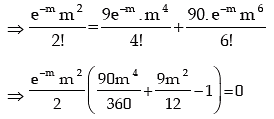
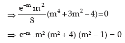
Solution: Let X be a Poisson variate with parameter m. Then the probability mass function of X is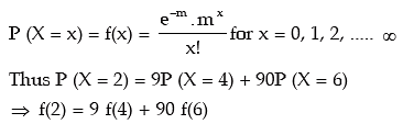




Example: Between 9 and 10 AM, the average number of phone calls per minute coming into the switchboard of a company is 4. Find the probability that during one particular minute, there will be,
1. no phone calls
2. at most 3 phone calls (given e–4 = 0.018316)
Solution: Let X be the number of phone calls per minute coming into the switchboard of the company. We assume that X follows Poisson distribution with parameters m = average number of phone calls per minute = 4.
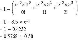
1. The probability that there will be no phone call during a particular minute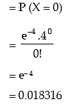

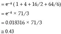
2. The probability that there will be at most 3 phone calls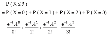


Example: If 2 per cent of electric bulbs manufactured by a company are known to be defectives, what is the probability that a sample of 150 electric bulbs taken from the production process of that company would contain 1. exactly one defective bulb? 2. more than 2 defective bulbs?
Solution: Let x be the number of bulbs produced by the company. Since the bulbs could be either defective or non-defective and the probability of bulb being defective remains the same, it follows that x is a binomial variate with parameters n = 150 and p = probability of a bulb being defective = 0.02. However since n is large and p is very small, we can approximate this binomial distribution with Poisson distribution with parameter m = np = 150 x 0.02 = 3.
1. The probability that exactly one bulb would be defective


2. The probability that there would be more than 2 defective bulbs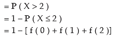


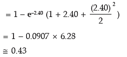
Example: The manufacturer of a certain electronic component is certain that two per cent of his product is defective. He sells the components in boxes of 120 and guarantees that not more than two per cent in any box will be defective. Find the probability that a box, selected at random, would fail to meet the guarantee? Given that e^–2.40 = 0.0907. Solution: Let x denote the number of electric components. Then x follows binomial distribution with n = 120 and p = probability of a component being defective = 0.02. As before since n is quite large and p is rather small, we approximate the binomial distribution with parameters n and p by a Poisson distribution with parameter m = n.p = 120 × 0.02 = 2.40. Probability that a box, selected at random, would fail to meet the specification = probability that a sample of 120 items would contain more than 2.40 defective items.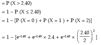


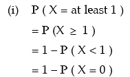
Example: A discrete random variable x follows Poisson distribution. Find the values of
(i) P (X = at least 1)
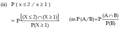
(ii) P (X ≤ 2/ X ≥ 1) You are given E (x) = 2.20 and e^–2.20 = 0.1108.
Solution: Since X follows Poisson distribution, its probability mass function is given by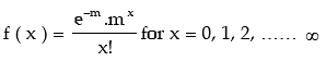





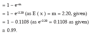
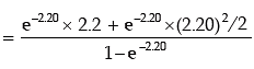 ( ∵ m = 2.2)

Fitting a Poisson distribution
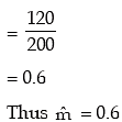
As explained earlier, we can apply the method of moments to fit a Poisson distribution to an observed frequency distribution. Since Poisson distribution is uniparametric, we equate m, the parameter of Poisson distribution, to the arithmetic mean of the observed distribution and get the estimate of m.

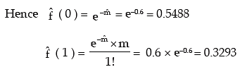
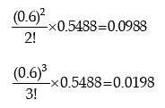
The fitted Poisson distribution is then given by

Example: Fit a Poisson distribution to the following data:

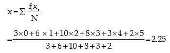
Solution: The mean of the observed frequency distribution is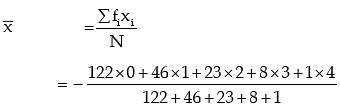




Lastly P ( X ≤ 4 ) = 1 – P ( X < 4 ).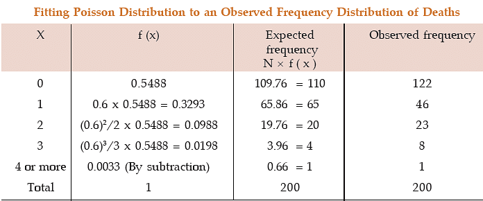


NORMAL OR GAUSSIAN DISTRIBUTION
The two distributions discussed so far, namely binomial and Poisson, are applicable when the random variable is discrete. In case of a continuous random variable like height or weight, it is impossible to distribute the total probability among different mass points because between any two unequal values, there remains an infinite number of values. Thus a continuous random variable is defined in term of its probability density function f (x), provided, of course, such a function really exists, f (x) satisfies the following condition:

The most important and universally accepted continuous probability distribution is known as normal distribution. Though many mathematicians like De-Moivre, Laplace etc. contributed towards the development of normal distribution, Karl Gauss was instrumental for deriving normal distribution and as such normal distribution is also referred to as Gaussian Distribution. A continuous random variable x is defined to follow normal distribution with parameters μ and σ², to be denoted by

If the probability density function of the random variable x is given by
 
where μ and σ are constants, and σ > 0 Some important points relating to normal distribution are listed below:
(a) The name Normal Distribution has its origin some two hundred years back as the then mathematician were in search for a normal model that can describe the probability distribution of most of the continuous random variables.
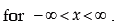
b) If we plot the probability function y = f (x), then the curve, known as probability curve, takes the following shape:
Showing Normal Probability Curve
A quick look at figure 17.1 reveals that the normal curve is bell shaped and has one peak, which implies that the normal distribution has one unique mode. The line drawn through x = μ has divided the normal curve into two parts which are equal in all respect. Such a curve is known as symmetrical curve and the corresponding distribution is known as symmetrical distribution. Thus, we find that the normal distribution is symmetrical about x = μ. It may also be noted that the binomial distribution is also symmetrical about p = 0.5. We next note that the two tails of the normal curve extend indefinitely on both sides of the curve and both the left and right tails never touch the horizontal axis. The total area of the normal curve or for that any probability curve is taken to be unity i.e. one. Since the vertical line drawn through x = μ divides the curve into two equal halves, it automatically follows that,
The area between –∞ to μ = the area between μ to ∞ = 0.5
When the mean is zero, we have
the area between –∞ to 0 = the area between 0 to ∞ = 0.5
(c) If we take μ = 0 and σ = 1 in (18.17), we have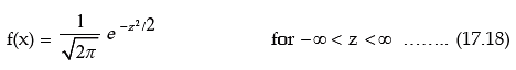

The random variable z is known as standard normal variate (or variable) or standard normal deviate. The probability that a standard normal variate X would take a value less than or equal to a particular value say X = x is given by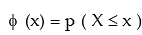

ϕ (x) is known as the cumulative distribution function. We also have ϕ (0) = P ( X ≤ 0 ) = Area of the standard normal curve between – ∞ and 0 = 0.5 …….. (17.20)
(d) The normal distribution is known as biparametric distribution as it is characterised by two parameters μ and σ². Once the two parameters are known, the normal distribution is completely specified.
Properties of Normal Distribution 
1. Since π = 22/7 , e^–θ = 1 / e^θ > 0, whatever θmay be,
it follows that f (x) ≥ 0 for every x.
It can be shown that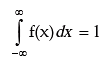

2. The mean of the normal distribution is given by μ. Further, since the distribution is symmetrical about x = μ, it follows that the mean, median and mode of a normal distribution coincide, all being equal to μ.
3. The standard deviation of the normal distribution is given by σ  Mean deviation of normal distribution is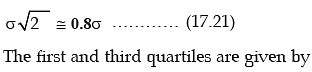


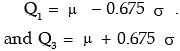
so that, quartile deviation = 0.675 σ
4. The normal distribution is symmetrical about x = μ . As such, its skewness is zero i.e. the normal curve is neither inclined move towards the right (negatively skewed) nor towards the left (positively skewed).
5. The normal curve y = f (x) has two points of inflexion to be given by x = μ – σ and x = μ + σ i.e. at these two points, the normal curve changes its curvature from concave to convex and from convex to concave.
6. If x ~ N ( μ , σ² ) then 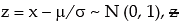is known as standardised normal variate or normal deviate. We also have P (z ≤ k ) = ϕ (k)
The values of ϕ(k) for different k are given in a table known as “Biometrika.”
Because of symmetry, we have
ϕ(– k) = 1 – ϕ(k)
We can evaluate the different probabilities in the following manner: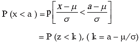

= ϕ(k)
Also P ( x ≤ a ) = P ( x < a ) as x is continuous.
P ( x > b ) = 1 – P ( x ≤ b )
= 1 – ϕ ( b – μ/σ )
and P ( a < x < b ) = ϕ ( b – μ/σ ) – ϕ ( a – μ/σ )
ordinate at x = a is given by
(1/σ) ϕ (a – μ/ σ)
Also, ϕ (– k) = ϕ (k)
The values of ϕ (k) for different k are also provided in the Biometrika Table.
7. Area under the normal curve is shown in the following figure :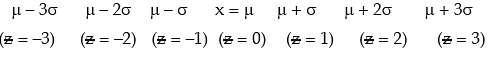

Area Under Normal Curve
From this figure, we find that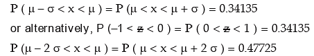


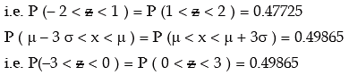
combining these results, we have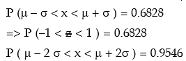


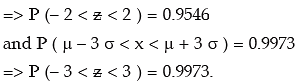
We note that 99.73 per cent of the values of a normal variable lies between (μ – 3 σ) and (μ + 3 σ). Thus the probability that a value of x lies outside that limit is as low as 0.0027.
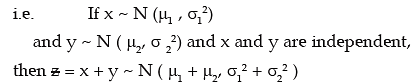
8. If x and y are independent normal variables with means and standard deviations as μ₁ and μ₂ and σ₁, and σ₂ respectively, then  also follows normal distribution with mean (μ_{1 +} μ₂ ) and SD