Electric Field due to Continuous Charge Distribution | Physics Class 12 - NEET PDF Download
Introduction
With the help of Coulomb’s Law and Superposition Principle, we can easily find out the electric field due to the system of charges or discrete system of charges. The word discrete means every charge is different and has the existence of its own. Suppose, a system of charges having charges as q1, q2, q3……. up to qn. We can easily find out the net charge by adding charges algebraically and net electric field by using the principle of superposition.
This is because:
- Discrete system of charges is easier to solve
- Discrete system of charges do not involve calculus in calculations

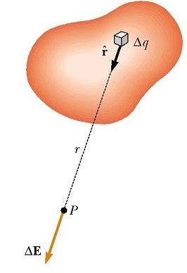
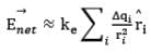 Considering the charge distribution as continuous, the total field at P in the limit Δqi → 0 is
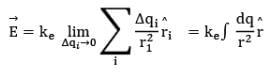
This means a combination of infinite point charges kept together forming a linear, surface or a volumetric shape constitutes a continuous charge system with linear, surface or volumetric charge density respectively.
Refer to the following figure: Thus, there are three types of continuous charge distribution system.
1. Linear Charge Distribution: A body having a finite charge distributed along its length i.e. along one dimension will have a linear charge distribution. In this case, we define the Linear Charge Distribution denoted by lower case Greek letter lambda (λ). Observe the rod given above of length L, a charge of +Q is distributed along the length of the rod. A small element dl will have a charge dq on itself. In this case, we define linear charge density of the rod.
dq = λdl [Charge on infinitely small element dl]
Q = ∫dq = ∫dl [Total charge on the rod]
2. Surface Charge Distribution: a body having a finite charge distributed along its area or surface will have a Surface Charge Distribution. In this case, we define the Surface Charge Distribution denoted by lower case Greek letter Sigma (σ).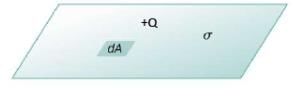

dq = σdA [Charge on infinitely small element d A]
Q = ∫dq = ∫σdA [Total charge on the sheet]
3. Volume Charge Distribution: a body having a finite charge distributed along its volume will have a Volumetric Charge Distribution. In this case, we define the Volumetric Charge Distribution denoted by lower case Greek letter rho (ρ).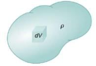

dq = ρdV [Charge on infinitely small volume element dV]
Q = ∫dq = ∫ρdV [Total charge on the body]
Linear Charge Density
When the charge is non-uniformly distributed over the length of a conductor, it is called linear charge distribution. It is also called linear charge density and is denoted by the symbol λ (Lambda).Mathematically linear charge density is λ = dq/dl
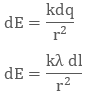
The unit of linear charge density is C/m. If we consider a conductor of length ‘L’ with surface charge density λ and take an element dl on it, then small charge on it will be
dq = λl
So, the electric field on small charge element dq will be
To calculate the net electric field we will integrate both sides with proper limit, that is
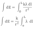
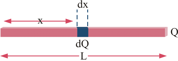
Fig: We take small element x and integrate it in case of linear charge density
Surface Charge Density
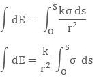
When the charge is uniformly distributed over the surface of the conductor, it is called Surface Charge Density or Surface Charge Distribution. It is denoted by the symbol σ (sigma) symbol and is the unit is C/m2.It is also defined as charge/ per unit area. Mathematically surface charge density is σ = dq/ds
where dq is the small charge element over the small surface ds. So, the small charge on the conductor will be dq = σds
The electric field due to small charge at some distance ‘r’ can be evaluated as

Integrating both sides with proper limits we get
Volume Charge Density
When the charge is distributed over a volume of the conductor, it is called Volume Charge Distribution. It is denoted by symbol ρ (rho). In other words charge per unit volume is called Volume Charge Density and its unit is C/m3. Mathematically, volume charge density is ρ = dq/dv
where dq is small charge element located in small volume dv. To find total charge we will integrate dq with proper limits. The electric field due to dq will be
dq = ρ dv

Integrating both sides with proper limits we get
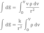
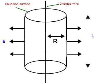
Fig: We can easily find electric field in different geometries using charge distribution system
Steps to calculate Electric Field Intensity due to continuous charge body:
(i) Identify the type of charge distribution and compute the charge density λ, σ or ρ.
(ii) Divide the charge distribution into infinitesimal charges dq, each of which will act as a tiny point charge.
(iii) The amount of charge dq, i.e., within a small element dl, dA or dV is
dq = λ dl (charge distributed in length)
dq = σ dA (charge distributed over a surface)
dq = ρ dV (charge distributed throughout a volume)
(iv) Draw at point P the dE vector produced by the charge dq. The magnitude of dE is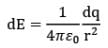
(v) Resolve the dE vector into its components. Identify any special symmetry features to show whether any component(s) of the field that are not canceled by other components.
(vi) Write the distance r and any trigonometric factors in terms of given coordinates and parameters.
(vii) The electric field is obtained by summing over all the infinitesimal contributions.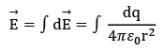
(viii) Perform the indicated integration over limit of integration that includes all the source charges.
Electric Field calculation due to Uniformly Distributed Continuous Charge
(a) Electric Field on axis of a uniformly charged circular ring: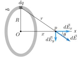 Consider a uniformly charged circular ring with a total charge +Q distributed uniformly along its length. We need to evaluate the net electric field due to this charged ring at a point P which is located x distance from its centre on its axis.
Conclude that the charge is distributed linearly throughout the length of the ring, hence we will define linear charge density λ for this ring,
λ = Total charge on the ring/𝑇otal Length =Q/2πr
Now, we consider an infinitely small length element dl on the ring,
Infinitesimal charge on element dl,
dq = λdl
Now, we write the expression of Electric Field at point P due to dq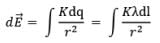
This, infinitely small electric field vector will be inclined at an angle θ with the axis of the ring (x axis), as shown in diagram.
We need to imagine components of  along the x and y axis i.e.
  and
and
By resolvingwe get,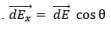
Observe and imagine, that will cancel out if we take each and every element of the ring into consideration.
Therefore net electric field at P,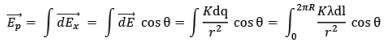
Now, by geometry,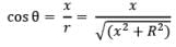
Thus,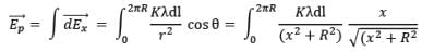
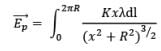
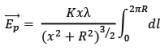
Replacing with the value of λ defined above,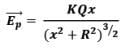
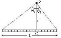
(b) Electric field strength at a general point due to a uniformly charged rod:
As shown in figure, if P is any general point in the surrounding of rod, to find the electric field strength at P, again we consider an element on rod of length dx at a distance x from point O as shown in figure.
Now if dE be the electric field at P due to the element, then it can be given as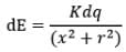
Here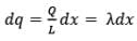
Now we resolve electric field in components. Electric field strength in x-direction due to dq at P is,
dEx = dEsin 𝜃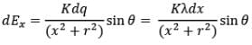
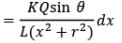
Here we have x = r tan 𝜃
and dx = rsec2 𝜃d𝜃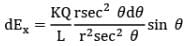
Net electric field strength due to dq at point P in x-direction is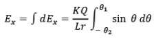
or 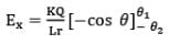
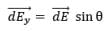
Similarly, the electric field strength at point P due to dq in y-direction is
dEy = dEcos𝜃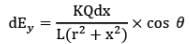
Again we have x = rtan 𝜃
And dx = rsec2 𝜃d𝜃
Thus we have,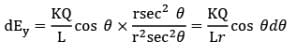
Net electric field strength at P due to dq in y-direction is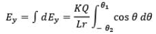
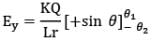
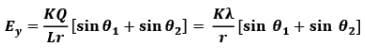
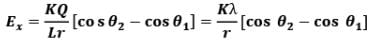
Thus electric field at a general point in the surrounding of a uniformly charged rod which subtends angles 𝜽1 and 𝜽2 at the two corners of the rod from the point of consideration can be given as In parallel direction,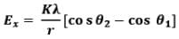
In perpendicular direction ,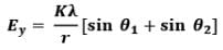
We can use this generalized finite relation to calculate the Electric Field due to following systems too:
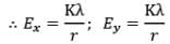
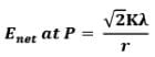
(i) Infinitely long uniformly charged rod with charge density 𝜆:
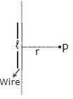
For infinite rod, 𝜃1 → 90° and 𝜃2 → 90°
Therefore, for infinitely long uniformly charged rod,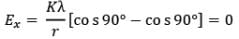
While,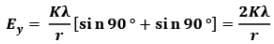
(ii) Electric field due to semi-infinite wire:
For this case,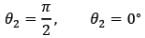
(c) Electric field strength due to a uniformly surface charged disc:
If there is a disc of radius R, charged on its surface with surface charge density s C/m2, we wish to find electric field strength due to this disc at a distance x from the centre of disc on its axis at point P shown in figure.
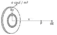
Note: Identify that the electric charge is distributed over the surface of the non-conducting disc, hence we would define a surface charge density σ for this disc.
σ = Total Charge/Total Area = Q/πR2
To find electric field at point P due to this disc, we consider an elemental ring of radius y and width dy in the disc as shown in figure. Now the charge on this elemental ring dq can be given as
dq = σ (dA)
where dA is the area of the ring element on the disc,
also we can imagine ring element to be a small rectangle with width dy. Thus,
dA = 2πydy
dq = σ(2πydy)
Now we know that electric field strength due to a ring of radius R. Charge Q at a distance x from its centre on its axis can be given as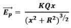
Here due to the elemental ring electric field strength dE at point P can be given as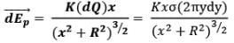
Net electric field at point P due to this disc is given by integrating above expression from O to R as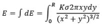
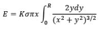
Now, using integration by substitution we can solve the above integral as,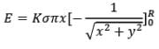
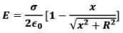
By geometry,
Hence,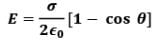
Please note that 𝜽 is the angle subtended by the disc at point P which is x distance far from the center.
Case: (i) If x < < R ⇒ cos 𝜽 → 1
Physically, this would mean that the disc has its radius R→ ∞, that is the disc can be effectively imagined as infinitely long sheet of charge,
Thus, Electric field due to infinitely long plane sheet of charge at a distance x would be,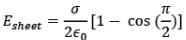
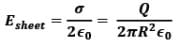
i.e. behaviour of the disc is like infinite sheet.
Case: (ii) If x > > R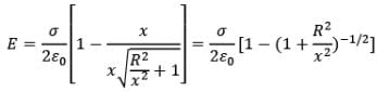
Now, using binomial approximation,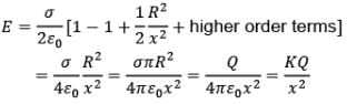
i.e. behaviour of the disc is like a point charge.
Electric Field Strength due to a uniformly charged Hollow Hemispherical Cup:
Figure shows a hollow hemisphere, uniformly charged with surface charge density 𝜎 C/m2 . To find electric field strength at its centre C, we consider an elemental ring on its surface of angular width dq at an angle q from its axis as shown. The surface area of this ring will be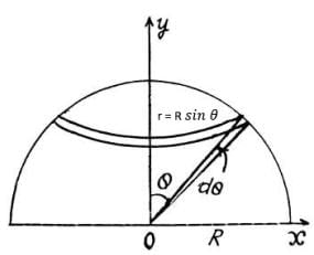 dA = 2𝜋r × Rdθ
By geometry, dA = 2𝜋R sin 𝜃 × Rdθ
Charge on this elemental ring is
dq = 𝜎d𝐴 = 𝜎. 2𝜋R sin 𝜃 × Rdθ
Now due to this ring electric field strength at centre C can be given as,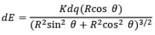
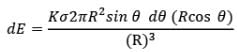
Net electric field at centre can be obtained by integrating this expression between limits 0 to 𝜋/2.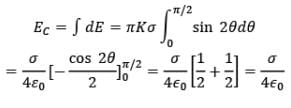
Hence, Electric Field intensity at centre C, due to uniformly charged nonconducting hemispherical shell is,
Above given continuous charged systems are most frequently used ones. It is recommended to remember the procedure and results by heart.
|
97 videos|336 docs|104 tests
|
FAQs on Electric Field due to Continuous Charge Distribution - Physics Class 12 - NEET
| 1. What is a continuous charge distribution? |  |
| 2. How is the electric field due to a continuous charge distribution calculated? | |
| 3. What is the relationship between charge density and electric field in a continuous charge distribution? | |
| 4. Can a continuous charge distribution have both positive and negative charges? | |
| 5. How does the shape of a continuous charge distribution affect the electric field? | |

|
4.80/5 Rating |

|
Dec 22, 2024 Last updated |

|
Explore Courses for NEET exam
|
|
shortcuts and tricks
,Viva Questions
,Semester Notes
,practice quizzes
,Extra Questions
,ppt
,mock tests for examination
,MCQs
,past year papers
,Objective type Questions
,Free
,Electric Field due to Continuous Charge Distribution | Physics Class 12 - NEET
,Important questions
,Sample Paper
,Previous Year Questions with Solutions
,Electric Field due to Continuous Charge Distribution | Physics Class 12 - NEET
,video lectures
,study material
,Exam
,Summary
,Electric Field due to Continuous Charge Distribution | Physics Class 12 - NEET
;


Electric Field due to Continuous Charge Distribution Free PDF Download
Importance of Electric Field due to Continuous Charge Distribution
Electric Field due to Continuous Charge Distribution Notes
Electric Field due to Continuous Charge Distribution NEET Questions
Study Electric Field due to Continuous Charge Distribution on the App
|
© EduRev
|
Education Revolution
|


|


