Lossless Decomposition

Lossless Join and Dependency Preserving Decomposition
A relation is decomposed when it is not in the desired normal form or when decomposition improves design by removing redundancy and update anomalies. A decomposition of a relation R into sub-relations R1, R2, ... must be checked for two important properties:
- Lossless join - the original relation R must be recoverable exactly by joining the decomposed relations.
- Dependency preserving - all functional dependencies (FDs) of R must be enforceable using the FDs that hold on the decomposed relations without requiring a join.
Lossless Join Decomposition
Let R be decomposed into R1 and R2. The decomposition is lossless if the natural join of R1 and R2 yields exactly R; otherwise it is lossy.
- Lossy decomposition: R1 ⋈ R2 ⊃ R
- Lossless decomposition: R1 ⋈ R2 = R
Using functional dependencies, a sufficient condition to ensure that a decomposition of R into R1 and R2 is lossless is:
- Att(R1) ∪ Att(R2) = Att(R). Every attribute of R appears in at least one of R1 or R2.
- Att(R1) ∩ Att(R2) ≠ ∅. The two projections share at least one attribute.
- The common attribute set must be a key for at least one of the projections. Formally, Att(R1) ∩ Att(R2) → Att(R1) or Att(R1) ∩ Att(R2) → Att(R2), where → denotes functional determination using the given FD set (or its closure).
Example: Let R(A, B, C, D) with FD set {A → BC}. Decompose into R1( A, B, C ) and R2( A, D ).
- Att(R1) ∪ Att(R2) = {A,B,C} ∪ {A,D} = {A,B,C,D} = Att(R).
- Att(R1) ∩ Att(R2) = {A} ≠ ∅.
- {A} → Att(R1) holds because A → BC is given, so A is a key of R1. Therefore the decomposition is lossless.
Dependency Preserving Decomposition
A decomposition D = {R1, R2, ..., Rn} of R is dependency preserving with respect to a set F of functional dependencies if the closure of the union of the projections of F onto each Ri is equal to F+. Formally, if Fi is the set of FDs that hold on Ri (projection of F onto Ri), then
(F1 ∪ F2 ∪ ... ∪ Fn)+ = F+.
Informally, every FD in F must be either present directly in some Ri or be inferable from the FDs that hold locally on the Ri without performing a join of the relations.
Example: Let R(A, B, C, D) and F = {A → B, C → D}. Decompose into R1( A, B ) and R2( C, D ).
- Att(R1) ∪ Att(R2) = {A,B} ∪ {C,D} = {A,B,C,D} = Att(R).
- Att(R1) ∩ Att(R2) = ∅, so the common-attribute condition for lossless join fails; hence the decomposition is not lossless.
- Each original FD is present in one of the projections: A → B is in R1 and C → D is in R2; therefore the decomposition is dependency preserving.
GATE Question
Q. Consider a schema R(A,B,C,D) and functional dependencies A->B and C->D. Then the decomposition of R into R1(AB) and R2(CD) is [GATE-CS-2001]
(a) dependency preserving and lossless join
(b) lossless join but not dependency preserving
(c) dependency preserving but not lossless join
(d) not dependency preserving and not lossless join
Ans: (c)
Solution: For lossless join decomposition, these three conditions must hold true:
- Att(R1) ∪ Att(R2) = ABCD = Att(R)
- Att(R1) ∩ Att(R2) = ∅, which violates the condition of lossless join decomposition.
Hence the decomposition is not lossless.
For dependency preserving decomposition, A → B is ensured in R1(AB) and C → D is ensured in R2(CD). Hence it is dependency preserving decomposition.
So, the correct option is C.
Dependency Preservation - Formal View and Example
Given R and F, the projection (or restriction) of F onto a sub-schema S (a subset of attributes of R) is the set of all functional dependencies X → Y such that X and Y are subsets of S and X → Y is implied by F. The decomposition is dependency preserving if the union of these projections implies F (i.e., no original FD is lost).
Worked Problem
Problem: Let R(A, B, C, D) and F = { AB → C, C → D, D → A }. Decompose R into R1(A, B, C) and R2(C, D). Check whether the decomposition is dependency preserving.
Solution:
Compute projection of F on R1 (attributes A,B,C):
C is in R1 and A is in R1, and C → D and D → A imply C → A (since C → D and D → A gives C → A by transitivity).
Therefore R1 yields the following FDs (implied by F and restricted to R1):
- AB → C (directly present in F and entirely in R1)
- C → A (implied by C → D and D → A and both C and A lie in R1)
- BC → A (follows from BC → C and C → A; projected because B,C,A are all in R1)
Compute projection of F on R2 (attributes C,D):
- C → D (directly present in F and entirely in R2)
Now consider the original set F = { AB → C, C → D, D → A }.
Check whether each FD in F is present or implied by F1 ∪ F2:
- AB → C is present in projection on R1.
- C → D is present in projection on R2.
- D → A is not present in either projection: D and A do not both belong to R2 (A is not in R2) and D → A is not implied by F1 ∪ F2 restricted to the attributes of decomposed relations.
Therefore F1 ∪ F2 does not imply D → A; the decomposition is not dependency preserving.
Finding Attribute Closure and Candidate Keys using Functional Dependencies
Functional Dependency - definition
A functional dependency X → Y holds in a relation R if for any two tuples t1 and t2 in R, whenever t1[X] = t2[X] then t1[Y] = t2[Y]. That is, X functionally determines Y.
Examples from an EMPLOYEE relation:
- E-ID → E-NAME holds if each E-ID corresponds to exactly one E-NAME.
- E-ID → E-CITY and E-CITY → E-STATE may hold as additional FDs.
- E-NAME → E-ID does not hold if multiple E-IDs share the same E-NAME.
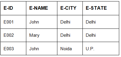 Table 1
The FD set for the EMPLOYEE relation in the example is:
{ E-ID → E-NAME, E-ID → E-CITY, E-ID → E-STATE, E-CITY → E-STATE }
Trivial and Non-trivial Functional Dependencies
A functional dependency X → Y is trivial if Y ⊆ X; such dependencies always hold. Otherwise the FD is non-trivial.
Example: {E-ID, E-NAME} → E-ID is trivial because the right side is contained in the left side. E-ID → E-NAME is non-trivial.
Armstrong's Axioms (Properties of FDs)
- Reflexivity: If Y ⊆ X then X → Y.
- Augmentation: If X → Y then XZ → YZ for any Z.
- Transitivity: If X → Y and Y → Z then X → Z.
- Attribute closure: The attribute closure of X, written X+, is the set of attributes functionally determined by X under F.
Computing Attribute Closure
Procedure to compute X+ given FD set F:
- Add X to X+.
- Repeatedly add any attribute A to X+ if there exists an FD Y → Z in F with Y ⊆ X+ and A ∈ Z.
- Stop when no new attributes can be added; the final set is X+.
Example: For R(E-ID, E-NAME, E-CITY, E-STATE) with F = { E-ID → E-NAME, E-ID → E-CITY, E-ID → E-STATE, E-CITY → E-STATE }:
Compute (E-ID)+ :
Add E-ID to the set: {E-ID}.
From E-ID → E-NAME, add E-NAME: {E-ID, E-NAME}.
From E-ID → E-CITY, add E-CITY: {E-ID, E-NAME, E-CITY}.
From E-ID → E-STATE (or from E-CITY → E-STATE once E-CITY is present), add E-STATE: {E-ID, E-NAME, E-CITY, E-STATE}.
Thus (E-ID)+ = {E-ID, E-NAME, E-CITY, E-STATE}.
Similarly (E-NAME)+ = {E-NAME}, and (E-CITY)+ = {E-CITY, E-STATE}.
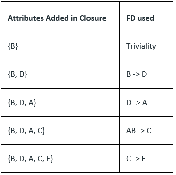
Worked exercise: Given R(ABCDE) with F = { AB → C, B → D, C → E, D → A }, compute closures such as (B)+ and (C,D)+.
- (C,D)+ : start with {C,D}.
- From C → E add E: {C, D, E}.
- From D → A add A: {A, C, D, E}.
- Therefore (C, D)+ = {A, C, D, E}.
- (B,C)+ : start with {B,C}.
- From B → D add D: {B, C, D}.
- From C → E add E: {B, C, D, E}.
- From D → A add A: {A, B, C, D, E}.
- Therefore (B, C)+ = {A, B, C, D, E} (the whole relation).
Candidate Keys and Superkeys
Superkey: Any set of attributes that functionally determines all attributes of the relation.
Candidate key: A minimal superkey - a superkey such that no proper subset is also a superkey.
Example: In the EMPLOYEE relation, E-ID is a candidate key because (E-ID)+ includes all attributes and no proper subset determines all attributes. Sets such as (E-ID, E-NAME) are superkeys but not candidate keys because they are not minimal.
Note: Every candidate key is a superkey, but not every superkey is a candidate key.
Practical Guidelines for Decomposition
- Prefer decompositions that are both lossless and dependency preserving. This preserves data correctness and allows enforcement of constraints locally.
- If trade-offs arise, lossless join is usually given higher priority than dependency preservation because a lossy decomposition leads to incorrect data when relations are joined.
- When dependency preservation is not possible, certain constraints will need to be enforced by checking across joins (which is more expensive at runtime).
- Use attribute closure and projection of FD algorithms to determine keys, losslessness, and dependency preservation precisely.
Summary
Lossless join ensures exact recoverability of the original relation from its decomposed parts. Dependency preserving decomposition ensures that all functional dependencies of the original relation can be enforced without expensive joins. Use attribute closure and FD projection to test these properties; when designing schemas aim for decompositions that satisfy both properties to maintain correctness and efficient constraint enforcement.
FAQs on Lossless Decomposition
| 1. What is lossless decomposition? |  |
| 2. Why is lossless decomposition important in database design? | |
| 3. How does lossless decomposition differ from lossy decomposition? | |
| 4. What are the advantages of lossless decomposition? | |
| 5. Can lossless decomposition be applied to any relation? | |


 | Explore Courses for Computer Science Engineering (CSE) exam |
 | Get EduRev Notes directly in your Google search |