AVL Tree


Introduction
Trees are fundamental data structures used to organise data for efficient search, insertion, and deletion. Real-world data sets change continuously; simple binary search trees can become skewed as elements are inserted or deleted, causing poor worst-case performance. A family of trees called height-balanced trees keeps tree height small by performing local adjustments during updates. An important example of a height-balanced binary search tree is the AVL tree.
Threaded binary trees are a different technique where NULL child links are replaced by special links (threads) to support traversals without recursion or an explicit stack. The AVL tree, by contrast, maintains balance by monitoring subtree heights and performing rotations when necessary. This chapter explains AVL trees: definition, balance factor, rotations, insertion and deletion algorithms, representation, complexity, and applications.
What is the AVL Tree?
An AVL tree is a binary search tree (BST) in which, for every node, the heights of its left and right subtrees differ by at most one. The technique was proposed by M. M. Adelson-Velskii and E. M. Landis (commonly cited together as Adelson-Velskii and Landis) in the early 1960s, and hence the name AVL.
Formally, let T be a non-empty binary tree with left subtree TL and right subtree TR. Tree T is height-balanced (an AVL tree) if:
- TL and TR are height-balanced, and
- |h(TL) - h(TR)| ≤ 1, where h(·) denotes subtree height.
The balance factor of a node is defined as:
balanceFactor(node) = height(node→left) - height(node→right)
The balance factor may take values -1, 0, or +1 for a balanced node. When the balance factor becomes less than -1 or greater than +1 for some node after an update, the subtree rooted at that node is unbalanced and must be rebalanced using rotations.
Advantages of AVL Trees
- AVL trees guarantee that the height is O(log n) for n nodes, so search, insertion and deletion operations take O(log n) time in the worst case.
- Because AVL trees are more strictly balanced than many other balanced trees, they have smaller height and therefore faster lookups on average for read-heavy workloads.
- Rotations used to restore balance are local operations and are easy to implement.
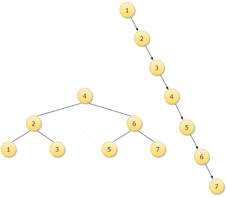
Consider inserting keys 1, 2, 3, 4, 5, 6, 7 into an ordinary BST in ascending order: the BST becomes a single long chain (linked list), producing O(n) search time. An AVL tree for the same insertion sequence will perform rotations to remain balanced and require far fewer comparisons for searches.
Representation of an AVL Tree
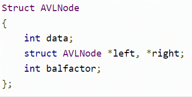
Each node in an AVL tree typically stores the key and pointers to left and right children. To support efficient balance updates, nodes also store the height of the subtree rooted at that node (or alternately the balance factor directly).
A typical node structure (illustrative, C-like) is:
Height and Balance Factor Calculation
The height of a NULL pointer is taken as 0 (or -1 in some conventions). Using the convention height(NULL) = 0, the height of a node is:
height(node) = 1 + max(height(node→left), height(node→right))
After any insertion or deletion, update heights for nodes on the path from the changed node up to the root and compute the balance factor for each node as:
balanceFactor(node) = height(node→left) - height(node→right)
If balanceFactor(node) ∈ {-1, 0, +1} the node is balanced. If it is outside this range, the node is unbalanced and requires rotations.
Rotations (Rebalancing Operations)
Rotations are local operations that restore the AVL property for an unbalanced subtree. There are four cases, classified by the direction of the imbalance:
- Left-Left (LL): A node is left-heavy (balance factor = +2) and its left child is left-heavy or balanced (balance factor ≥ 0). Perform a single right rotation.
- Right-Right (RR): A node is right-heavy (balance factor = -2) and its right child is right-heavy or balanced (balance factor ≤ 0). Perform a single left rotation.
- Left-Right (LR): A node is left-heavy and its left child is right-heavy. Perform a left rotation on the left child, then a right rotation on the node (double rotation).
- Right-Left (RL): A node is right-heavy and its right child is left-heavy. Perform a right rotation on the right child, then a left rotation on the node (double rotation).
Rotation details (single right rotation shown in words):
- Let x be the unbalanced node, y = x→left. Perform a right rotation around x so that y becomes the new root of the subtree, x becomes y→right, and y→right (if any) becomes x→left. Update heights of x and y after rotation.
All rotations preserve the binary search tree order and only rearrange pointers locally. Heights of only a few nodes change, so rotations are efficient O(1) operations.
Insertion into an AVL Tree
Insertion in an AVL tree proceeds as in a BST followed by rebalancing on the path from the insertion point back to the root.
- Insert the new key using standard BST insertion (place as a leaf).
- Walk back up to the root and update the heights of the visited nodes.
- For each visited node, compute its balance factor.
- If a node becomes unbalanced (balance factor < -1 or > +1), determine which of the four cases (LL, RR, LR, RL) applies by examining the balance factor of the child, and apply the corresponding rotation(s).
- After rotation(s), continue updating heights up the tree as required. At most one rebalance is needed at the lowest unbalanced ancestor to restore balance to the entire tree on insertion.
Example (conceptual): inserting keys 1, 2, 3 into an empty AVL tree.
Insert 1: becomes root.
Insert 2: goes to the right of 1; heights updated; balance factors remain within limits.
Insert 3: goes to the right of 2; node 1 has balance factor -2 (right-heavy) with right child having balance factor -1 ⇒ RR case ⇒ perform a left rotation at node 1. After rotation, 2 becomes root of subtree with 1 as left child and 3 as right child.
Deletion from an AVL Tree
Deletion in an AVL tree follows BST deletion semantics, then rebalances the tree on the path from the deletion point upward.
- Find the node containing the key (standard BST search).
- Delete the node using standard BST deletion rules:
- If the node has no children, remove it.
- If the node has one child, replace the node with its child.
- If the node has two children, find the node's in-order successor (smallest node in the right subtree), copy the successor's contents into the node, and delete the successor (which then has at most one child). This reduces deletion to removing a node with at most one child.
- Walk back up from the deleted node's parent to the root, updating heights and checking balance factors.
- If a node becomes unbalanced, identify the rotation case (LL, RR, LR, RL) based on its child's balance factor and perform the appropriate rotation(s).
- Continue this process up to the root; deletion may require multiple rebalances on the path to the root.
Note: After deletion, a subtree's height can decrease, so multiple ancestors may become unbalanced and need correction.
Time and Space Complexity
- Search: O(log n) worst-case, because AVL trees maintain height O(log n).
- Insertion: O(log n) worst-case; costs include BST insertion (O(log n)) plus at most O(1) rotations (constant-time) at the lowest unbalanced node; overall O(log n) due to height updates along the insertion path.
- Deletion: O(log n) worst-case; BST deletion followed by O(log n) possible rebalances along the path to root; still O(log n) overall.
- Space: O(n) for storing n nodes. Each node stores a height (or balance factor) value in addition to pointers.
Implementation Notes
- Store the height in each node to compute balance factors in O(1) time per node visited.
- When implementing rotations, always update heights of nodes whose subtrees changed, typically the two nodes involved in a single rotation or three in a double rotation.
- Carefully handle NULL pointers and the convention used for height(NULL) (commonly 0) to compute balance factors consistently.
- Test edge cases: inserting duplicates (decide whether duplicates are allowed and how to handle them), deleting root, rebalancing chains of nodes.
Applications and Comparison
- AVL trees are suitable for applications with many lookups and where strictly balanced trees are desirable for predictable fast searches.
- Compared with Red-Black trees, AVL trees are more rigidly balanced and often faster for lookups but may perform more rotations on inserts/deletes. Red-Black trees allow O(log n) operations with fewer rotations on average and are commonly used in library implementations (for example, map/set in some standard libraries).
- AVL trees are commonly taught in data-structures courses and are used in scenarios that prioritise read performance.
Summary
An AVL tree is a self-balancing binary search tree that enforces the invariant that heights of the left and right subtrees of every node differ by at most one. Balance is measured by the balance factor, and local rotations (LL, RR, LR, RL) restore balance after insertions and deletions. AVL trees guarantee O(log n) worst-case time for search, insert and delete, making them suitable for applications requiring efficient and predictable lookups.
FAQs on AVL Tree
| 1. What is an AVL Tree? |  |
| 2. What are the advantages of AVL Trees? | |
| 3. How is the height and balance factor calculated in an AVL Tree? | |
| 4. What are the types of rotations used in rebalancing an AVL Tree? | |
| 5. What are the time and space complexities of AVL Tree operations? | |


 | Explore Courses for Computer Science Engineering (CSE) exam |
 | Get EduRev Notes directly in your Google search |