Probability Distributions (Exponential Distribution)


Introduction
Suppose we are posed with the question - how much time do we need to wait before a given event occurs?
The answer can be given in probabilistic terms by modelling the waiting time as a random variable and using the exponential distribution. If the probability that the event occurs in any short interval is proportional to the length of that interval (and independent of the past), then the waiting-time random variable has an exponential distribution.
The support (set of values the random variable can take) of an exponential random variable is the set of all non-negative real numbers.
Support: Rx = [0, ∞)
Probability Density Function
For a positive real number λ the probability density function (pdf) of an exponentially distributed random variable X is
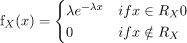
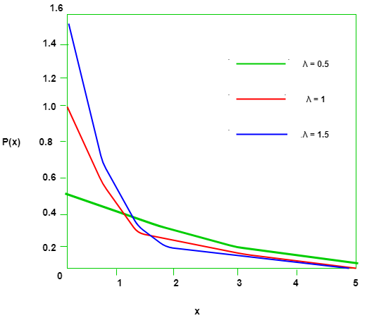
Here λ (lambda) is the rate parameter and λ > 0. Larger values of λ correspond to shorter typical waiting times; smaller λ correspond to longer waiting times.
To check that f(x) is a valid probability density function, we verify that its integral over the support equals 1.
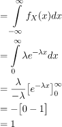
The integral equals 1 because
∫₀^∞ λ e-λx dx = λ [ -(1/λ) e-λx ]₀^∞ = 1.
Cumulative Distribution Function
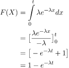
The cumulative distribution function (cdf) F(x) gives the probability that the random variable X is ≤ x. For the exponential distribution, for x ≥ 0,
Equivalently, the tail probability (survival function) is
P(X > x) = e-λx for x ≥ 0.
Expected Value
The expected value (mean) of X is obtained by integrating x times the pdf over the support.
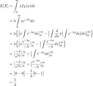
Thus
E[X] = 1 / λ.
Variance and Standard Deviation
The second moment about zero is E[X²] = 2 / λ² and hence the variance is
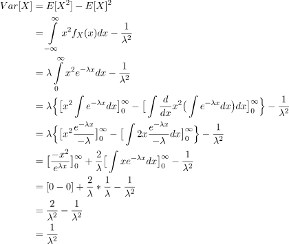
Therefore
Variance: Var(X) = 1 / λ².
Standard deviation: σ = 1 / λ.

Example: Let X denote the time between detections of a particle with a Geiger counter and assume that X has an exponential distribution with E(X) = 1.4 minutes. What is the probability that we detect a particle within 30 seconds of starting the counter?
Solution:
Given that the expected value E[X] = 1.4 minutes.
E[X] = 1 / λ
1 / λ = 1.4
λ = 1 / 1.4
Convert 30 seconds to minutes: 30 seconds = 0.5 minutes.
The probability of detecting a particle within 30 seconds is P(X ≤ 0.5) which equals the cdf at 0.5.
P(X ≤ 0.5) = 1 - e-λ(0.5)

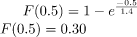
Substitute λ = 1 / 1.4 and evaluate to obtain the numerical probability.
Lack of Memory Property
The exponential distribution has the lack of memory (memoryless) property: for any s, t ≥ 0,
P(X > s + t | X > s) = P(X > t).
Equivalently,
Proof sketch:
P(X > s + t | X > s) = P(X > s + t) / P(X > s).
Using the tail form P(X > x) = e-λx, we get
P(X > s + t | X > s) = e-λ(s+t) / e-λs = e-λt = P(X > t).
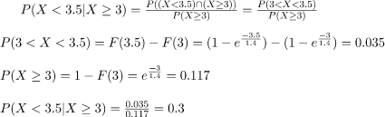
Thus, the probability of waiting at least an additional time t does not depend on how long one has already waited. In the Geiger counter example, if no particle is detected in the first 3 minutes, the probability of detecting a particle in the next 30 seconds is the same as it was at the start; past waiting does not change the future probability.
Applications and Remarks
The exponential distribution commonly models waiting times between independent events that occur at a constant average rate, for example:
- Time between arrivals in a Poisson process (electrical pulses, customers, failures).
- Lifetime of memoryless devices or components (where the hazard/rate is constant).
- Inter-arrival times used in queueing theory and reliability engineering.
Key properties to remember:
- Support: X ≥ 0.
- Pdf: f(x) = λ e-λx, x ≥ 0.
- Cdf: F(x) = 1 - e-λx, x ≥ 0.
- Mean: E[X] = 1 / λ.
- Variance: Var(X) = 1 / λ².
- Memoryless property: P(X > s + t | X > s) = P(X > t).
FAQs on Probability Distributions (Exponential Distribution)
| 1. What is the exponential distribution? |  |
| 2. How is the exponential distribution characterized? | |
| 3. What is the cumulative distribution function (CDF) of the exponential distribution? | |
| 4. How is the exponential distribution related to the Poisson process? | |
| 5. What are some real-world applications of the exponential distribution? | |


