Probability Distributions (Normal Distribution)

Introduction
Whenever a random experiment is repeated many times, the random variable that equals the average (or total) result over the replicates tends to follow a normal distribution as the number of replicates becomes large. This phenomenon is a cornerstone of probability theory and statistics because of the Central Limit Theorem. Many real-world quantities (for example, measurement errors, physical characteristics, test scores) are approximately normally distributed. The normal distribution is also known as the Gaussian distribution or the bell-shaped distribution.
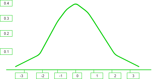
The graph above shows a distribution that is symmetric about its centre, which is also the mean (0 in this case). Because of symmetry, values at equal distances on either side of the mean have equal probability density. The density is highly concentrated near the mean and decreases for values further from the mean.
Probability Density Function
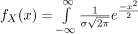
The probability density function (pdf) of the general normal distribution is

In the formula above, μ denotes the mean and σ denotes the standard deviation (so variance = σ²). The pdf defines the relative likelihood of the continuous random variable taking a given value.
The z-score measures how many standard deviations a value x is away from the mean μ. It is given by

The exponent in the pdf is -(z-score)²/2. Hence values far from the mean (with larger |z|) receive much smaller densities, while values near the mean (small |z|) have higher density. This quantitative form explains the bell shape and concentration of probability near μ.
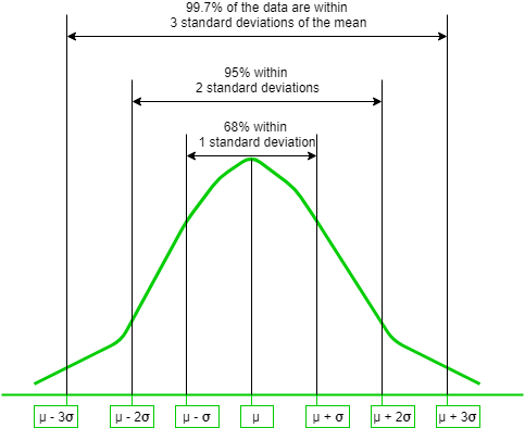
The empirical 68-95-99.7 rule summarises the concentration for a normal distribution:
- Approximately 68% of values lie within ±1σ of the mean.
- Approximately 95% of values lie within ±2σ of the mean.
- Approximately 99.7% of values lie within ±3σ of the mean.
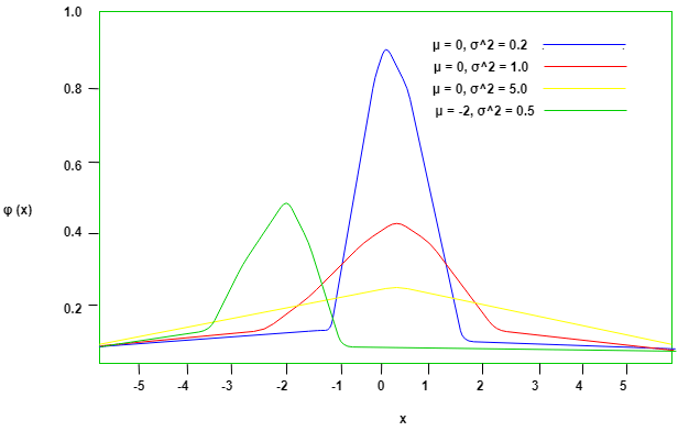
The parameters μ and σ affect the graph as follows: μ shifts the centre of the curve left or right; σ controls the spread (larger σ produces a flatter, wider curve; smaller σ produces a taller, narrower curve).
Expectation and Variance
Let X be a normally distributed random variable with mean μ and variance σ². The expected value and variance can be obtained by integrating the pdf. The derivation is presented in clear steps.
X has pdf f(x) equal to the normal pdf shown above.
Expected value E[X] is defined by the integral of x times the pdf over all real x.
Write x as (x - μ) + μ.
The integral for E[X] splits into two integrals: one involving (x - μ) and one involving μ.
The integral of (x - μ) times the symmetric pdf about μ is 0 because the integrand is an odd function about μ.
The integral of μ times the pdf is μ times 1 (since the total area under the pdf is 1).
Therefore E[X] = μ.


To find the variance, compute E[(X - μ)²]. For the normal distribution this integral evaluates to σ². Thus
Variance Var(X) = σ².
Standard deviation = σ.

Standard Normal Distribution
If μ = 0 and σ = 1, the normal distribution obtained is called the standard normal distribution. Its pdf is
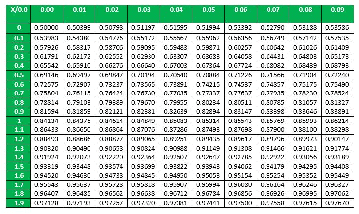
The cumulative distribution function (cdf) of the normal distribution does not have a simple closed-form expression in elementary functions. Practical work therefore uses precomputed standard normal tables or software. To use a table for a general normal variable X ~ N(μ, σ²), we standardize X to the standard normal Z and then use the table values.
This approach is beneficial for two reasons:
- Only one table (for the standard normal) is required to handle all normal distributions.
- The table size is limited because the 68-95-99.7 rule implies that nearly all probability mass lies within ±3σ of the mean; therefore beyond about z = ±3 cumulative probabilities are approximately 0 or 1.
If X is normal with E[X] = μ and Var(X) = σ², then the random variable

is standard normal with E[Z] = 0 and Var(Z) = 1. In words, Z = (X - μ)/σ.
Example
Suppose that the current measurements in a strip of wire are assumed to follow a normal distribution with a mean of 10 milliamperes and a variance of four (milliamperes)². What is the probability that a measurement exceeds 13 milliamperes?
Solution:
Let X denote the current in milliamperes.
X ~ N(10, 4).
We want the probability P(X > 13).
Standardize X to Z by using
Z = (X - 10)/2.
Then
P(X > 13) = P(Z > (13 - 10)/2).
P(X > 13) = P(Z > 1.5).
From the standard normal table, P(Z ≤ 1.5) = 0.93319.
P(Z > 1.5) = 1 - 0.93319 = 0.06681.
Summary for the Standard Normal
For the standard normal random variable Z ~ N(0,1):
- Expected value E[Z] = 0.
- Variance Var(Z) = 1.
- Standard deviation = 1.
Remarks, Applications and Notes for Engineering Students
- The normal distribution is central to statistical inference (confidence intervals, hypothesis tests) because many estimators converge to normality by the Central Limit Theorem.
- In civil engineering, normal models are used for measurement errors, material property variations, and load uncertainties (when many small independent effects contribute).
- In electrical engineering, noise sources are often modelled as Gaussian; the additive white Gaussian noise (AWGN) model is fundamental in communications.
- In computer science and data analysis, many algorithms assume approximately normal residuals; standardisation (z-scores) is commonly used for feature scaling.
- When using standard normal tables, always check whether the table gives P(Z ≤ z) or P(0 ≤ Z ≤ z) and adjust calculations accordingly.
- Software (R, Python, MATLAB) provides accurate functions for pdf, cdf and quantiles of the normal distribution and removes the need for manual table lookup in practical problems.
FAQs on Probability Distributions (Normal Distribution)
| 1. What is a normal distribution? |  |
| 2. How is the normal distribution characterized? | |
| 3. What is the empirical rule for the normal distribution? | |
| 4. How can the normal distribution be used in statistics? | |
| 5. Can real-world data always be modeled by a normal distribution? | |