Probability Distributions (Poisson Distribution)

Introduction
Suppose an event can occur several times within a given unit of time. When the total number of occurrences of the event is unknown, we treat it as a discrete random variable. A commonly used model for such counts is the Poisson distribution. The Poisson distribution often arises as a limiting case of the Binomial distribution when the number of trials is large and the probability of success in each trial is small, while the expected number of successes remains finite.
For a Binomial experiment with n trials and success probability p, the probability of exactly x successes is
P(X = x) = C(n,x) px(1 - p)n - x
If n → ∞ and p → 0 in such a way that λ = np remains fixed, the Binomial probability tends to the Poisson probability with parameter λ. The Poisson distribution is therefore appropriate for modelling rare events occurring in a large number of small opportunities.
Probability Mass Function (PMF)
The Poisson distribution with parameter λ > 0 has probability mass function
P(X = x) = e-λ λx / x!, x = 0, 1, 2, ...
Here, λ is the expected number of occurrences in the unit interval (or unit region) under consideration. The PMF satisfies the normalisation condition Σx=0∞ P(X = x) = 1 because the series for eλ converges.
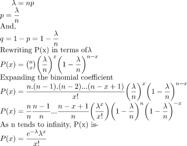
Derivation as Limit of the Binomial Distribution
Derive the Poisson PMF from the Binomial PMF by setting λ = np and letting n → ∞, p → 0.
Start with the Binomial probability:
C(n,x) px(1 - p)n - x
Rewrite using λ = np and p = λ/n:
C(n,x) (λ/n)x (1 - λ/n)n - x
Use C(n,x) = n(n - 1) ... (n - x + 1) / x! and observe that as n → ∞, n(n - 1) ... (n - x + 1) / nx → 1. Also (1 - λ/n)n → e-λ and (1 - λ/n)-x → 1.
Thus the limit becomes
e-λ λx / x!.
Hence the Poisson PMF follows as the limiting form.
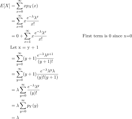
Expected Value
The expected value (mean) of a Poisson random variable X ∼ Poisson(λ) is λ. A direct derivation is:
Start from the definition
E[X] = Σx=0∞ x e-λ λx / x!.
Note that the x = 0 term is zero, so change the summation index by writing x = k + 1.
E[X] = e-λ Σx=1∞ x λx / x!.
Rewrite the term x / x! as 1 / (x - 1)! and change the index:
E[X] = e-λ Σk=0∞ λk+1 / k!.
Factor λ outside the sum:
E[X] = λ e-λ Σk=0∞ λk / k!.
Recognise the series for eλ:
E[X] = λ e-λ eλ = λ.
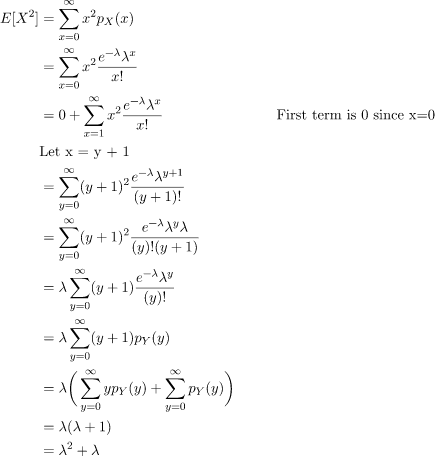
Variance and Standard Deviation
The variance of a Poisson random variable equals its mean, so Var(X) = λ. A common derivation uses the factorial moment E[X(X - 1)].
First compute E[X(X - 1)]:
E[X(X - 1)] = Σx=0∞ x(x - 1) e-λ λx / x!.
Remove the first two zero terms and change the index to show that
E[X(X - 1)] = λ2.
Then use E[X2] = E[X(X - 1)] + E[X].
Therefore E[X2] = λ2 + λ.
Now compute the variance:
Var(X) = E[X2] - (E[X])2 = (λ2 + λ) - λ2 = λ.
The standard deviation is
σ = √Var(X) = √λ.
Relation with the Exponential Distribution and Poisson Process
The Poisson distribution is closely connected with the Poisson process. A counting process {N(t), t ≥ 0} is called a Poisson process with rate λ if it satisfies the following properties:
- Independent increments: numbers of events occurring in disjoint time intervals are independent.
- Stationary increments: the distribution of the number of events in an interval depends only on the length of the interval, not on its location.
- Probability of a single event in a very small interval of length h is approximately λh, and the probability of two or more events in that interval is negligible (o(h)).
Under these conditions, the count N(t) over interval of length t is Poisson distributed with parameter λt.
The time between successive events (interarrival time) in a Poisson process is independent and identically distributed with an Exponential(λ) distribution. Conversely, if the successive interarrival times are independent exponential random variables with rate λ, then the counting process of arrivals is a Poisson process and the number of arrivals in any interval of length t is Poisson(λt).
The exponential distribution is memoryless, which matches the independent increments property of the Poisson process.
Applications in Engineering
- Civil Engineering: modelling the number of cracks or defects per unit length or area; rare event counts in quality control and material testing.
- Computer Science & Information Technology: modelling packet arrivals in networks, number of errors in blocks of data, requests to a server in unit time.
- Electrical Engineering: modelling arrival of noise pulses, failures of components per unit time, counts in reliability and telecommunication traffic.
- General engineering uses: queues (arrival processes), reliability (failures in a time window), and spatial counts (points per unit area) when events are random and rare.
Example
Example: For the case of the thin copper wire, suppose that the number of flaws follows a Poisson distribution with a mean of 2.3 flaws per millimeter. Determine the probability of exactly two flaws in 2 millimeter of wire.
Solution:
Let X denote the number of flaws in 1 millimetre of wire.
The expected number of flaws in 1 millimetre is λ1 = 2.3.
For 2 millimetres the expected number is λ = 2 × λ1 = 2 × 2.3 = 4.6.
For a Poisson random variable with parameter λ, the probability of exactly two occurrences is
P(X = 2) = e-λ λ2 / 2!.
Substitute λ = 4.6 into the formula:
P(X = 2) = e-4.6 (4.6)2 / 2!.
Compute the numerical value (calculator may be used):
4.62 = 21.16.
2! = 2.
P(X = 2) = e-4.6 × 21.16 / 2 = 10.58 × e-4.6.
Using e-4.6 ≈ 0.010041 (approx.),
P(X = 2) ≈ 10.58 × 0.010041 ≈ 0.1062 (approx.).

Summary
The Poisson distribution models counts of rare events in a fixed interval. Its PMF is P(X = x) = e-λ λx / x!, and it satisfies E[X] = Var(X) = λ. The distribution arises as a limit of the Binomial distribution under suitable conditions and is intimately connected with the Poisson process and exponential interarrival times. It is widely used across civil, computer and electrical engineering for modelling defects, arrivals, failures and other count data.
FAQs on Probability Distributions (Poisson Distribution)
| 1. What is a Poisson distribution? |  |
| 2. How is the Poisson distribution different from other probability distributions? | |
| 3. What are the characteristics of a Poisson distribution? | |
| 4. In what situations can the Poisson distribution be applied? | |
| 5. How is the Poisson distribution used in practice? | |


