Introduction: Divide & Conquer


Introduction
In this chapter we study the Divide and Conquer technique: a general algorithm design paradigm that breaks a problem into smaller subproblems, solves the subproblems (often recursively), and then combines the solutions to obtain a solution to the original problem. The topics covered are:
- Introduction to Divide and Conquer.
- Standard algorithms that apply the technique.
- Recurrence relations that express the running time of Divide and Conquer algorithms and methods to solve them.
- Worked example(s) and implementations.
Divide and Conquer
The Divide and Conquer technique splits a problem into independent subproblems, solves each subproblem recursively, and then combines the subsolutions. The technique is structured in three main steps:
- Divide: Split the original problem into two or more smaller subproblems of the same type.
- Conquer: Solve each subproblem recursively. If a subproblem is small enough, solve it directly (base case).
- Combine: Merge the solutions of the subproblems to produce a solution to the original problem.
When to use Divide and Conquer
Use Divide and Conquer when a problem can be naturally split into multiple independent subproblems whose solutions can be combined efficiently. If the same subproblems are recomputed many times, dynamic programming or memoization is usually preferable.
Standard Algorithms that Use Divide and Conquer
- Quicksort: A comparison sort that picks a pivot element, partitions the array so that elements less than the pivot come to its left and elements greater come to its right, then recursively sorts the left and right partitions. Average time complexity O(n log n); worst-case O(n²) without randomisation or careful pivot choice.
- Merge Sort: The array is divided into two halves, each half is sorted recursively, and the two sorted halves are merged. Time complexity O(n log n) in all cases; stable sort.
- Closest Pair of Points: Given n points in the plane, the brute-force O(n²) method checks all pairs. A Divide and Conquer algorithm computes the closest pair in O(n log n) time by splitting points by x-coordinate, recursively finding closest pairs in halves, and checking a strip around the split line.
- Strassen's Matrix Multiplication: A faster matrix multiplication algorithm than the naive O(n³) method. Strassen reduces the number of multiplications using a Divide and Conquer scheme to obtain time ≈ O(n^{log₂7}) ≈ O(n^{2.8074}).
- Cooley-Tukey Fast Fourier Transform (FFT): A Divide and Conquer method to compute the discrete Fourier transform in O(n log n) time by splitting the sequence into even and odd indices and combining results with twiddle factors.
- Karatsuba Multiplication: A Divide and Conquer algorithm for multiplying large integers. It multiplies two n-digit numbers using at most 3 multiplications of numbers with about n/2 digits, giving time O(n^{log₂3}) ≈ O(n^{1.585}). For n = 2¹⁰ = 1024, the exact count of recursive multiplications is 3^{10} = 59,049 compared with the classical (grade-school) count of (2^{10})² = 1,048,576 single-digit multiplications.
What Does Not Qualify as Divide and Conquer
Binary Search is often mistaken for Divide and Conquer, but it is a case of Decrease and Conquer. In binary search each recursive step produces only one subproblem (the left half or the right half), not multiple independent subproblems. Divide and Conquer normally requires two or more independent subproblems per step.
Generic Divide and Conquer Algorithm and Recurrence Relation
A generic outline of a Divide and Conquer algorithm looks like this:
function DAC(problem): if problem is small: return direct solution divide the problem into subproblems for each subproblem: solve subproblem recursively combine subsolutions and return result
Typical recurrence for the running time T(n) when a problem of size n is split into a subproblems each of size n/b, with additional work f(n) spent in dividing and combining, is:
T(n) = a · T(n/b) + f(n)
For many standard algorithms, a and b are constants (for example, Merge Sort has a = 2 and b = 2), so the recurrence simplifies to:
T(n) = 2 T(n/2) + f(n)
Master Theorem (summary)
The Master Theorem gives asymptotic solutions for recurrences of the form T(n) = a T(n/b) + f(n), where a ≥ 1 and b > 1 are constants and f(n) is an asymptotically positive function.
- If f(n) = O(n^{log_b a - ε}) for some ε > 0, then T(n) = Θ(n^{log_b a}).
- If f(n) = Θ(n^{log_b a} · log^k n) for some k ≥ 0, then T(n) = Θ(n^{log_b a} · log^{k+1} n).
- If f(n) = Ω(n^{log_b a + ε}) for some ε > 0, and if a · f(n/b) ≤ c · f(n) for some c < 1 and sufficiently large n (regularity condition), then T(n) = Θ(f(n)).
Apply this theorem to common recurrences: for Merge Sort, a = 2, b = 2 and f(n) = Θ(n), so log_b a = 1 and T(n) = Θ(n log n).
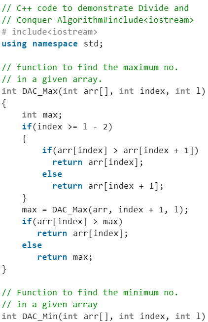
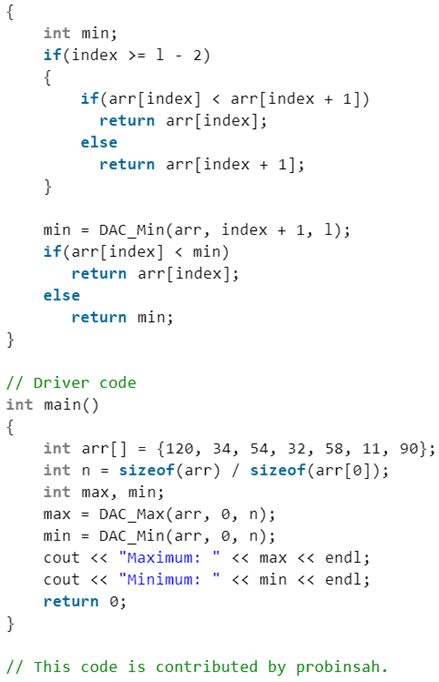
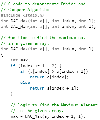
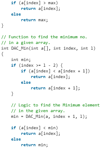
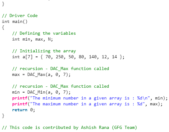
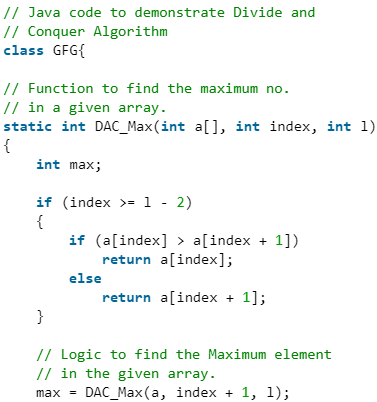
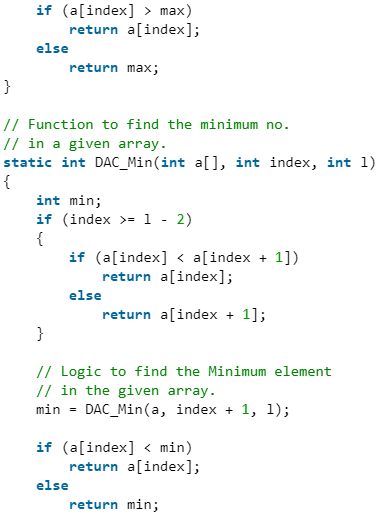
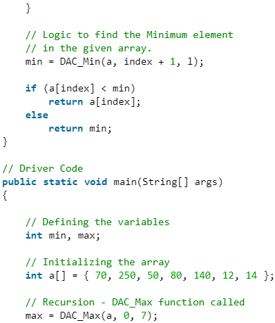
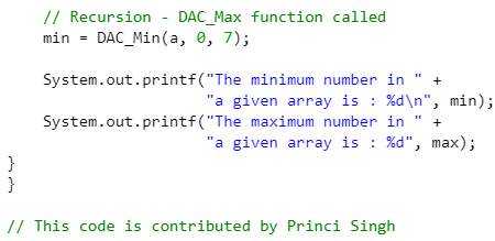
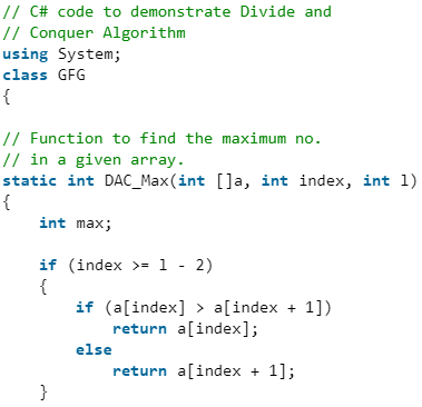
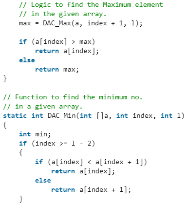
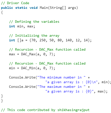
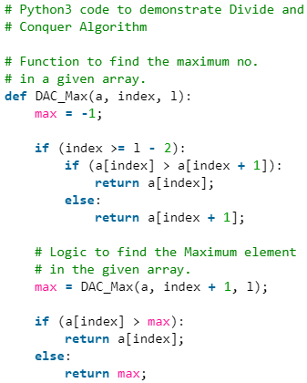
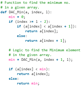
Example: Finding Minimum and Maximum in an Array
Problem statement: Given an array, find the minimum and maximum elements.
Input example: { 70, 250, 50, 80, 140, 12, 14 }
Expected output for this input:
- The minimum number in the given array is: 12
- The maximum number in the given array is: 250
Divide and Conquer approach (description)
We use a Divide and Conquer scheme that divides the array into two halves, recursively finds min and max for each half, and then combines the two results by taking the min of the two minima and the max of the two maxima. This approach performs O(n) comparisons overall, but can be arranged to use at most 3n/2 - 2 comparisons (optimal in the comparison model) using pairwise comparisons.
Algorithm (pseudocode)
function MinMax(A, left, right): if left == right: return (A[left], A[left]) // one element: min = max = A[left] if right == left + 1: if A[left] < A[right]: return (A[left], A[right]) // two elements: compare once else: return (A[right], A[left]) mid = floor((left + right) / 2) (minL, maxL) = MinMax(A, left, mid) (minR, maxR) = MinMax(A, mid+1, right) minAll = min(minL, minR) maxAll = max(maxL, maxR) return (minAll, maxAll)
Step-wise explanation and complexity
Procedure of the algorithm:
The array is divided into two halves recursively until subarrays of size 1 or 2 are reached.
For a subarray of size 1, we return that element as both min and max in constant time.
For a subarray of size 2, we perform one comparison and return min and max accordingly.
After obtaining min and max from left and right halves, we perform two comparisons to compute overall min and max.
Recurrence for running time (number of comparisons roughly follows the same recurrence):
T(n) = 2 T(n/2) + O(1)
Applying the Master Theorem with a = 2, b = 2 and f(n) = O(1) gives T(n) = Θ(n).
Optimised comparison count: arranging comparisons in pairs and using a suitable base-case handling leads to at most 3n/2 - 2 comparisons for n ≥ 2.
Implementation
Below are placeholders for implementations in several languages. Each image placeholder represents code or screenshots; preserve these placeholders as anchors for the implementations.
C++
C
Java
C#
Python3
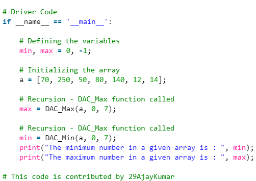
Sample program output
For a suitable input the program prints the computed maximum and minimum values. For the example earlier the output is:
- Maximum: 250
- Minimum: 12
Divide and Conquer (D & C) versus Dynamic Programming (DP)
Both paradigms subdivide problems, but the choice between them depends on whether subproblems overlap.
- Divide and Conquer should be used when subproblems are independent and not recomputed many times. Examples include Merge Sort and Quicksort.
- Dynamic Programming is the preferred approach when the same subproblems occur multiple times (overlapping subproblems) and the problem exhibits optimal substructure. Use memoization or bottom-up tabulation to avoid redundant work; an example is computing Fibonacci numbers efficiently.
Summary
Divide and Conquer is a fundamental algorithm design technique. Write recurrences to express running times, and use tools such as the Master Theorem to solve them. Recognise when subproblems overlap-if they do, prefer Dynamic Programming or memoization; otherwise, Divide and Conquer is usually the right choice. Common examples of Divide and Conquer include Merge Sort, Quicksort, FFT, Strassen's matrix multiplication and Karatsuba multiplication.
FAQs on Introduction: Divide & Conquer
| 1. What is Divide & Conquer in Computer Science Engineering (CSE)? |  |
| 2. How does Divide & Conquer approach work in CSE? | |
| 3. What are the key steps involved in the Divide & Conquer algorithm? | |
| 4. What are the advantages of using the Divide & Conquer technique in CSE? | |
| 5. What are some examples of algorithms that use the Divide & Conquer technique in CSE? | |


 | Explore Courses for Computer Science Engineering (CSE) exam |
 | Get EduRev Notes directly in your Google search |