Overlapping Subproblems Property in Dynamic Programming | Algorithms - Computer Science Engineering (CSE) PDF Download
Introduction
Dynamic Programming is an algorithmic paradigm that solves a given complex problem by breaking it into subproblems and stores the results of subproblems to avoid computing the same results again. Following are the two main properties of a problem that suggests that the given problem can be solved using Dynamic programming.
Property of Dynamic Programming
- Overlapping Subproblems
- Optimal Substructure
1. Overlapping Subproblems
Like Divide and Conquer, Dynamic Programming combines solutions to sub-problems. Dynamic Programming is mainly used when solutions of same subproblems are needed again and again. In dynamic programming, computed solutions to subproblems are stored in a table so that these don’t have to be recomputed. So Dynamic Programming is not useful when there are no common (overlapping) subproblems because there is no point storing the solutions if they are not needed again. For example, Binary Search doesn’t have common subproblems. If we take an example of following recursive program for Fibonacci Numbers, there are many subproblems which are solved again and again.
Recursion tree for execution of fib(5)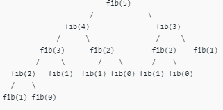
We can see that the function fib(3) is being called 2 times. If we would have stored the value of fib(3), then instead of computing it again, we could have reused the old stored value. There are following two different ways to store the values so that these values can be reused:
(i) Memoization (Top Down)
(ii) Tabulation (Bottom Up)
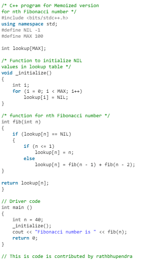
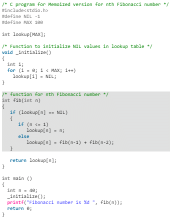
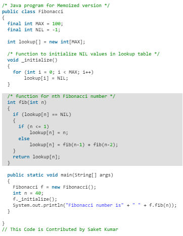
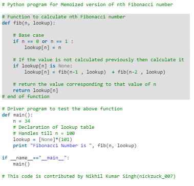
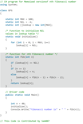
(i) Memoization (Top Down): The memoized program for a problem is similar to the recursive version with a small modification that it looks into a lookup table before computing solutions. We initialize a lookup array with all initial values as NIL. Whenever we need the solution to a subproblem, we first look into the lookup table. If the precomputed value is there then we return that value, otherwise, we calculate the value and put the result in the lookup table so that it can be reused later.
Following is the memoized version for nth Fibonacci Number:
- C++

- C

- Java

- Python

- C#

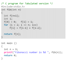
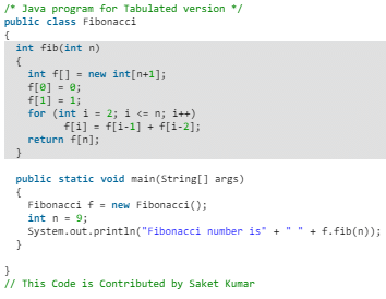
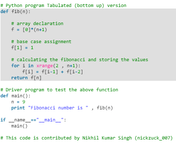
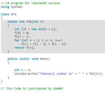
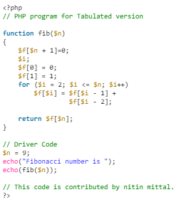
(ii) Tabulation (Bottom Up): The tabulated program for a given problem builds a table in bottom up fashion and returns the last entry from table. For example, for the same Fibonacci number, we first calculate fib(0) then fib(1) then fib(2) then fib(3) and so on. So literally, we are building the solutions of subproblems bottom-up.
Following is the tabulated version for nth Fibonacci Number:
- C/C++

- Java

- Python

- C#

- PHP

Output: Fibonacci number is 34
Both Tabulated and Memoized store the solutions of subproblems. In Memoized version, table is filled on demand while in Tabulated version, starting from the first entry, all entries are filled one by one. Unlike the Tabulated version, all entries of the lookup table are not necessarily filled in Memoized version. For example, Memoized solution of the LCS problem doesn’t necessarily fill all entries.
To see the optimization achieved by Memoized and Tabulated solutions over the basic Recursive solution, see the time taken by following runs for calculating 40th Fibonacci number:
- Recursive solution
- Memoized solution
- Tabulated solution
Time taken by Recursion method is much more than the two Dynamic Programming techniques mentioned above – Memoization and Tabulation!
Also, see method 2 of Ugly Number post for one more simple example where we have overlapping subproblems and we store the results of subproblems.
2. Optimal Substructure
A given problems has Optimal Substructure Property if optimal solution of the given problem can be obtained by using optimal solutions of its subproblems.
For example, the Shortest Path problem has following optimal substructure property:
If a node x lies in the shortest path from a source node u to destination node v then the shortest path from u to v is combination of shortest path from u to x and shortest path from x to v. The standard All Pair Shortest Path algorithms like Floyd–Warshall and Bellman–Ford are typical examples of Dynamic Programming.
On the other hand, the Longest Path problem doesn’t have the Optimal Substructure property. Here by Longest Path we mean longest simple path (path without cycle) between two nodes. Consider the following unweighted graph given in the CLRS book. There are two longest paths from q to t: q→r→t and q→s→t. Unlike shortest paths, these longest paths do not have the optimal substructure property. For example, the longest path q→r→t is not a combination of longest path from q to r and longest path from r to t, because the longest path from q to r is q→s→t→r and the longest path from r to t is r→q→s→t.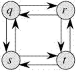
|
81 videos|80 docs|33 tests
|

|
Explore Courses for Computer Science Engineering (CSE) exam
|

|
