Functions of One Variable - I | Mathematics for Competitive Exams PDF Download

Introduction
Function
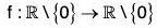
If A and B two non-empty sets then a relation defined from A to B is said to be a function if every element of A is associated with some unique element of set B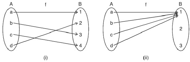
Domain, Co-domain & Range
If y = f(x) is a function such that f is defined from A B then
- Domain:Set A is called domain of f(x) and it is the set from which the independent variable ‘x’ takes its values. The independent variables ‘x’ must be able to take each and every element of set A
- Co-domain:Set B is called co-domain of f(x) and it is the set from which the dependent variable y takes its values the dependent variables ‘y’ cannot take its values outside the co-domain.
- Range:The set of values that y actually takes for different values of ‘x' is called range of f(x)
⇒ Range is a subset of B Range ⊆ co - domain
Real-valued Function
A function whose range is in the real numbers is said to be a real-valued function, also called a real function.
Example 1: f(x) = 1/x a real-valued function,
Sol: Each member of the codomain of f(x) =
is a real number.
Also note that excluding zero from the codomain does not change the fact that every other member is a real number. Symbolically, we have
Sinceis a subset of
then the expression above can be read as f is a real-valued function of a real-valued variable.
Example 2: The function f, g, and h defined on (-∞, ∞) by
Sol: f(x) = x2, g(x) = sin x, and h(x) = ex
have ranges [0, ∞), [-1, 1], and (0, ∞), respectively.
Example 3: The equation
Sol: [f(x)]2 = x ...(1)
does not define a function except on the singleton set {0}. If x < 0, no real number satisfies (1), while if x > 0, two real numbers satisfy (1). However, the conditions
[f(x)]2 = x and f(x) > 0
define a function f (1) Df = [0, ∞) with values f(x) = √x . Similarly, the conditions
[g(x)]2 = x and g(x) < 0
define a function g on Dg = (-∞, 0] with values g(x) = - √x . The ranges of f and g are [0, ∞) and (-∞, 0], respectively.
Arithmetic Operations on Functions
If Df ∩ Dg ≠ 0, then f + g, f - g and fg are defined by
(f + g)(x) = f(x) + g(x),
(f - g)(x) = f(x) - g(x),
and
(fg)(x) = f(x)g(x).
The quotient f/g is defined by
for x in Df ∩ Dg such that g(x) ≠ 0.
Example 1: If f(x) =  and g(x) =
  then Df = [- 2 , 2] and Dg = [1, ∞), so f + g, f - g, and fg are defined on Df ∩ Dg = [1, 2] by
Sol: (f + g)(x) =
(f - g)(x) =
and...(2)
The quotient f/g is defined on (1, 2] by
Although the last expression in (2) is also defined for -∞ < x < -2, it does not represent fg for such x, since g is not defined on (-∞, -2] but f is.
Example 2: If c is a real number, the function cf defined by (cf)(x) = cf(x) can be regarded as the product of f and a constant function. Its domain is Df. The sum and product of n (> 2) functions f1,.....fn are defined by
Sol: (f1 + f2 + ... + fn) (x) = f1(x) + f2(x) + ... + fn(x)
and
(f1 + f2 + ... + fn)(x) = f1(x) * f2(x) * ... * fn(x) ...(3)
onprovided that D is nonempty. If f1 = f2 = ... = fn, then (3) defines the nth power of f :
(fn)(x) = (f(x))n.
From these definitions, we can build the set of all polynomials
p(x) = a0 + a1x + ... + anxn,
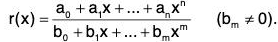
starting from the constant functions and f(x) = x. The quotient of two polynomials is a rational function
The domain of r is the set of points where the denominator is nonzero.
Domain of Definition
The domain on which the function is define is known as domain of definition.
[let y = f(x) be a rule, D subset of R on which f becomes real valued function, i.e. if f :D → R with D subset of R then D is called Dod - domain of definition
Ex- f(x) = (1/x), Dod ~ R-{0}
Ex- f(x) = logex, Dod ~ R+]
Types of Functions
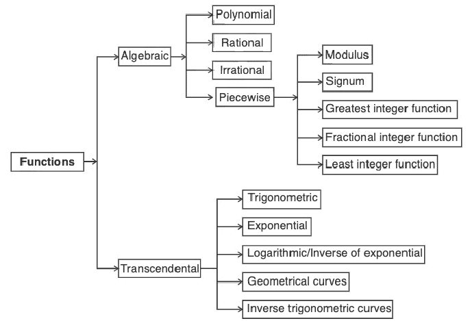
Algebraic Functions
Polynomial Function A function of the form :
- f(x) = a0 + a1x + a2x2 + ... + anxn ;
where n ∈ N and a0, a1, a2, ..., an ∈
- Then, f is called a polynomial function . “f(x) is also called polynomial in x” .
Some of basic polynomial functions are
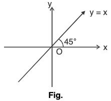
(i) Identity function/Graph of f(x) = x
- A function f defined by f(x) = x for all x ∈
 is called the identity function.
 - Here, y = x clearly represents a straight line passing through the origin and inclined at an angle of 45° with x-axis shown as : The domain and range of identity functions are both equal to

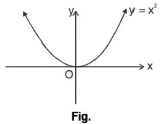
 (ii) Graph of f(x) = x2
- A function given by f(x) = x2 is called the square function.
- The domain of square function is
 and its range is
  ∪ {0} or [0, ∞)
 - Clearly y = x2, is a parabola. Since y = x2 is an even function, so its graph is symmetrical about y-axis, shown as :
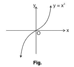
(iii) Graph of f(x) = x3
- A function given by f(x) = x3 is called the cube function.
- The domain and range of cube are both equal to

- Since, y = x3 is an odd function, so its graph is symmetrical about opposite quadrant, i.e., “origin”,shown as :
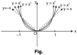
(iv) Graph of f(x) = x2n; n ∈ N
- If n ∈ N, then function f given by f(x) = x2n is an even function.
- So, its graph is always symmetrical about y-axis.
Also, x2 > x4 > x6 > x8 > ... for all x ∈ (-1,1)
and x2 < x4 < x6 < x8 < ... for all x ∈ (-∞,-1) υ(1,∞) - Graphs of y = x2, y = x4, y = x6,..., etc. areshownas:
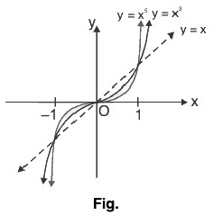
(v) Graph of f(x) = x2n-1; n ∈ N
- If n ∈ N, then the function f given by f(x) = x2n-1 is an odd function. So, its graph is symmetrical about origin or opposite quadrants.
- Here, comparison of values of x, x3, x5, ...
x ∈ (1, ∞)x<x3<x5<...
x ∈ (0, 1)x>x3>x5>...
x ∈ (-1, 0)x<x3<x5< ...
x ∈ (-∞, -1)x>x3>x5>... - Graphs of f(x) = x, f(x) = x3, f(x) = x5, ... are shown as in Fig.
Rational Function
A function obtained by dividing a polynomial by an other polynomial is called a rational function.
Domain ∈ - {x | Q(x) = 0}
i.e. domain ∈ except those points for which denominator = 0.
Graphs of some Simple Rational Functions
(i) Graph of f(x) = 1/x
- A function defined by f(x) = 1/x is called the reciprocal function or rectangular hyperbola, with coordinate axis as asymptotes. The domain and range of f(x) = 1/x is
 - {0}.
Since, f(x) is odd function, so its graph issymmetrical about opposite quadrants. Also, we observe
and as x → ± ∞ ⇒ f(x) → 0.
Thus, could be shown as in Fig.
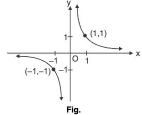
(ii) Graph of f(x) = 1/x2
- Here,
 is an even function, so its graph issymmetrical about y-axis.
Domain of f(x) is - {0} and range is (0, ∞).
Also, as y → ∞ as
Thus, could be shown as in Fig.
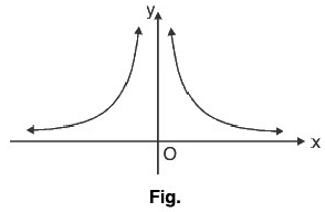
(iii) Graph of f(x) = 
- Here, f(x) =
 is an odd function, so its graph is Symmetrical in opposite quadrants.
Also, y → when f(x) and y → - ∞ when
Thus, the graph for f(x) = etc. will be similar to the graph of f(x) = 1/x which has asymptotes as coordinate axes, shown as in Figure.
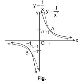
(iv) Graph of f(x) = 
- We observe that the function f(x) =
 is an even function, so its graph is symmetrical about y-axis.
As, y → ∞ as f(x) or
 f(x)
f(x)
and y → 0 as f(x) or
 f(x).
f(x).
The values of y decrease as the values of x increase. Thus, the graph of f(x) =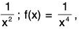 etc. will be similar as the graph of f(x) = 1/x2, which has asymptotes as coordinate axis. Shown as in Fig.
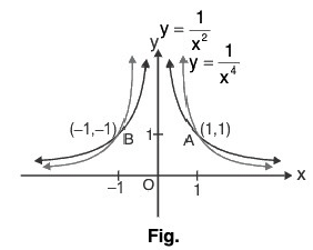
Irrational Function
The algebraic function containing terms having non-integral rational powers of x are called irrational functions.
Graphs of Some Simple Irrational Functions
(i) Graph of f(x) = x1/2
- Here, f(x) = √x is the portion of the parabola y2 = x, which lies above x-axis.
Domain of f(x) ∈ R+ u {0} or [0, ∞)
and range of f(x) ∈ R+ u {0} or [0, ∞)
Thus, the graph of f(x) = x1/2 is shown as;
If f(x) = xn and g(x) = x1/n, then f(x) and g(x) are inverse of each other.
∴ f(x) = xn and g(x) = x1/n is the mirror image about y = x.
(ii) Graph of f(x) = x1/3
- As discussed above, if g(x) = x3. Then f(x) = x,1/3 is image of g(x) about y = x. wheredomain f(x) ∈ R.
andrange of f(x) ∈ R.
Thus, the graph of f(x) = x1/3 is shown in Fig.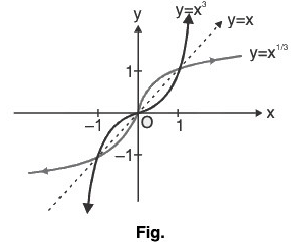
(iii) Graph of f(x) = x1/2n; n e N
- Here f(x) = x1/2n is defined for all x e [0, ∞) and the values taken by f(x) are positive.
So, domain and range of f(x) are [0, ∞).
Here, the graph of f(x) = x,/2n is the mirror image of the graph of f(x) = x2n about the line y = x, when x e [0, oo).
Thus, f(x) = x1/2, f(x) = x1/4, ... are shown as;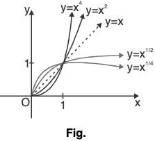
(iv) Graph of f(x) = x1/2n-1when n ∈ N
- Here, f(x) = x1/2n-1 is defined for all x ∈
 So, domain of f(x) ∈ R, and range of f(x) ∈ R. Also the graph of f(x) = x,1/2n-1 is the mirror image of the graph of f(x) = x2n-1 about the line y = x when x ∈
Thus, f(x) = x1/3, f(x) = x1/5, are shown as;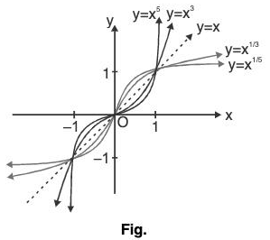
Piecewise Functions
As discussed piecewise functions are:
(i) Absolute value function (or modulus function)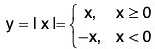
“It is the numerical value of x”.
“It is symmetric about y-axis" where domain ∈ 
and range ∈ [0, ∞).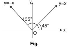
Properties of modulus functions
- I x I < a - a < x < a ; (a > 0)
- lxl > a => x < -a or x > a ; (a > 0)
- lx ± y| < l x l + l y l
- I x ± y | > II x I - | y ||
(ii) Signum function; y = Sgn(x)
It is defined by;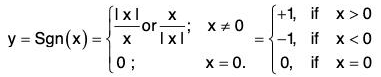
Here, Domain of f(x) ∈
and Range of f(x) ∈ {-1, 0, 1}.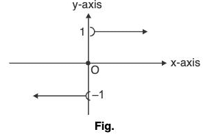
Greatest integer function
[x] indicates the integral part of x which is nearest and smaller integer to x. It is also known as floor of x.
Thus, [2, 3] = 2, [0.23] = 0, [2] = 2, [-8.0725] = -9
In general; n < x < n + 1(n ∈ Integer) ⇒ [x] = n.
Here, f(x) = [x] could be expressed graphically as;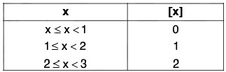
Thus, f(x) = [x] could be shown as;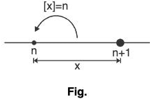
Properties of greatest integer function
- [x] = x holds, if x is integer.
- [x + I] = [x] + I, if I is integer.
- [x + y] > [x] + [y].
- If [ϕ(x)] > I, then ϕ (x) > I.
- If [ϕ(x)] < I, then ϕ(x) <1 + 1.
- [-x] = -[x], if x ∈ integer.
- [-x] = -[x] -1, if x ∉ integer.
“It is also known as stepwise function/floor of x.”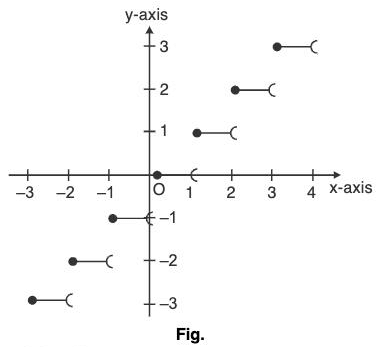 Fractional part of function
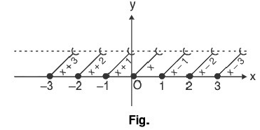
Here, {.} denotes the fractional part of x. Thus, in y = {x}.
x = [x] + {x} = I + f ; where I = [x] and f = {x}
y = {x} = x - [x], where 0 < {x} < 1; shown as: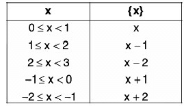
Properties of fractional part of x
- {x} = x ; if 0 < x < 1
- {x} = 0 ; if x e integer.
- {-x} = 1 - {x} ; if x e integer.
Least Integer Function
y = (x)= M.
(x) or x I indicates the integral part of x which is nearest and greatest integer to x.
It is known as ceiling of x.
Thus, [2.3023] = 3, (0.23) = 1, (-8.0725) = - 8, (-0.6) = 0
In general, n < x < n + 1 (n ∈ integral))
i.e., [x] or (x) = n + 1
shown as;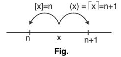 Here, f(x) = (x) = [x], can be expressed graphically as:
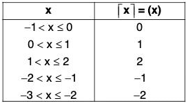
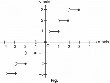 Properties of least integer function
- (x) = [x] = x, if
- (x + I) = I x + I 1 = (x) = I ; if I ∈ integer.
- Greatest integer converts x = I + f to [x] = I while (xl converts to (I + 1).
Transcendental Functions
Trigonometric Function
(a) Sine Function: Here, f(x) = sin x can be discussed in two ways i.e., Graph diagram and Circle diagram where Domain of sine function is  and range is [-1, 1].
Graph Diagram
(On x-axis and y-axis)
f(x) = sin x, increases strictly from - 1 to 1 as x increases from  decreases strictly from 1 to -1 as x increases from
  and so on. We have graph as;
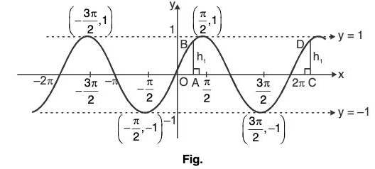 Here, the height is same after every interval of 2k. (i.e., In above figure, AB = CD after every interval of 2n).
sin x is called periodic function with period 2n.
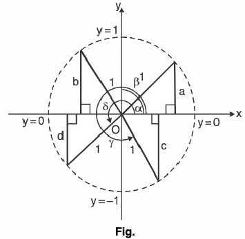
Circle Diagram
(On trigonometric plane or using quadrants). Let a circle of radius T, i.e., unit circle.
Then, 
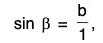

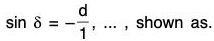
∴ sin x generates a circle of radius '1'.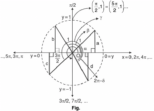 (b) Cosine Function: Here, f(x) = cos x
The domain of cosine function is R and the range is [-1, 1].
Graph diagram (on x-axis and y-axis)
As discussed, cos x decreases strictly from 1 to -1 as x increases from 0 to π, increases strictly from -1 to 1 as x increases from π to 2π and so on. Also, cos x is periodic with period 2k.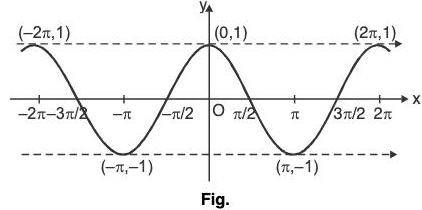 Circle Diagram
Let a circle of radius '1', i.e., a unit circle.
∴ cos x generates a circle of radius '1'.
(c) Tangent Function: f(x) = tan x
The domain of the function y = tan x is;
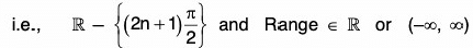
The function y = tan x increases strictly from - oo to + oo as x increases from
The graph is shown as :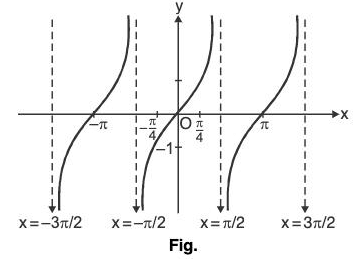 Note : Here, the curve tends to meet at x =
  ...but never meets or tends to infinity.
∴  are asymptotes to y = tan x.
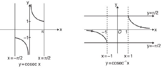
(d) Cosecant Function: f(x) = cosec x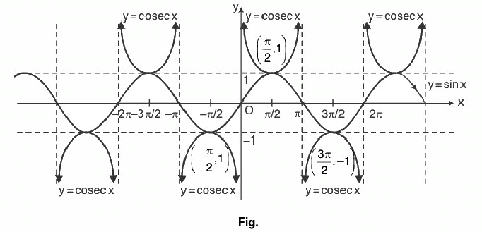 Here, domain of y = cosec x is,
R - {0, ±π, ±2π, ±3π, ...}
i.e., R - {nπ I n ∈ z} and range e  - (- 1, 1)
as shown in Fig.
The function y = cosec x is periodic with period 2π.
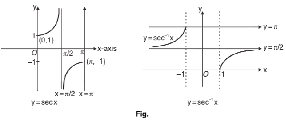
(e) Secant Function: f(x) = sec x
Here, 
Range ∈ R - (-1, 1)
Shown as:
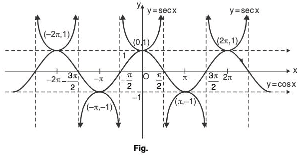 The function y = sec x is periodic with period 2n.
- The curve y = cosec x tends to meet at x = 0, ±π, ±2π, ... at infinity.
∴ = 0, ±π, ±2π, ...
or x = nπ, n ∈ integer are asymptote to y = cosec x. - The curve y = sec x tends to meet at x =
 ... at infinity.
 n ∈ integer are asymptote to y = cosec x.
(f) Cotangent Function: f(x) = Cot x
Here, domain ∈  - {nπ In ∈ z} Range ∈ R.
which is periodic with period π, and has x = nπ, n ∈ z as asymptotes. As shown in Fig.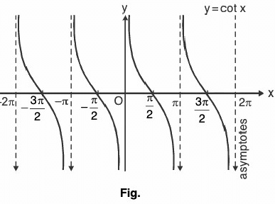
Exponential Function
Here, f(x) = ax, a > 0, a ≠ 1, and x ∈ R, where domain ∈ 
Range ∈ (0, ∞).
Case I. a > 1
Here, f(x) = y = ax increase with the increase in x, i.e., f(x) is increasing function on R.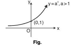
For Ex;
y = 2x y = 3x, y = 4x, ... have;
2x < 3x < 4x < ... for x > 1
and2x > 3x > 4x > ... for 0 < x < 1.
and they can be shown as;
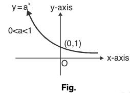
Case II. 0 < a < 1
Here, f(x) = ax decrease with the increase in x, i.e., f(x) is decreasing function on R.
“In general, exponential function increases or decreases as (a > 1) or (0 < a < 1) respectively”.
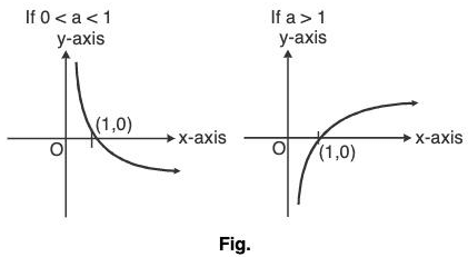
Logarithmic Function
(Inverse of Exponential)
The function f(x) = loga x; (x, a > 0) and a ≠ 1 is a logarithmic function.
Thus, the domain of logarithmic function is all real positive numbers and their range is the set R of all real numbers.
We have seen that y = ax is strictly increasing when a > 1 and strictly decreasing when 0 < a < 1.
Thus, the function is invertible.The inverse of this function is denoted by loga x, we write
y = ax ⇒ x = loga y;
where x ∈ R and y e (0, ∞) writing y = loga x in place of x = loga y, we have the graph of y =loga x.
Thus, logarithmic function is also known as inverse of exponential function.
Properties of logarithmic function
- loge (ab) = loge a + loge b {a, b > 0}
-
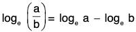 {a, b > 0}
 - loge am = m loge a {a > 0 and m ∈ R }
- loga a = 1 {a > 0 and a ≠ 1}
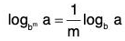 {a, b > 0, b * 1 and m e R}
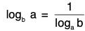 {a, b > 0 and a, b ≠ 1}
 {a, b > 0 * {1} and m > 0}
 {a, m > 0 and a ≠ 1}
 {a, b, c > 0 and c ≠ 1}
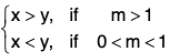
- If logm x > logm y ⇒
which could be graphically shown as;
If m > 1 (Graph of logm a)
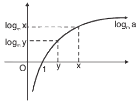
⇒ logm x > logm y when x > y and m > 1.
Again if 0 < m < 1. (Graph of logm a)
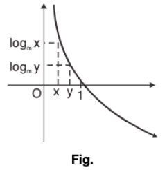
⇒ logm x > logm y; when x < y and m < m < 1.
- logm a = b ⇒ a = mb { a , m > 0 ; m * 1; b ∈ R }
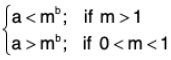
- logm a > b ⇒
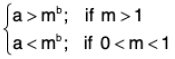
- logm a < b ⇒
Geometrical Curves
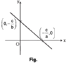
(a) Straight line : ax + by + c = 0 (represents general equation of straight line). We know,
y = -c/b where x = 0
and x = -c/a where y = 0
joining above points we get required straight line.
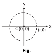
(b) Circle : We know,
(i) x2 + y2 = a2 is circle with centre (0, 0) and radius r.
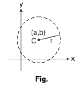
(ii) (x - a)2 + (y - b)2 = r2, circle with centre (a, b) and radius r.
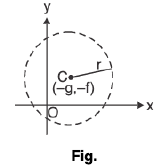
(iii) x2 + y2 + 2gr + 2fy + c = 0; centre (-g, -f); radius 
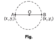
(iv) (x - x1)(x - x2) + (y - y1)(y - y2) = 0;
End points of diameter are (x1, y1) and (x2, y2).
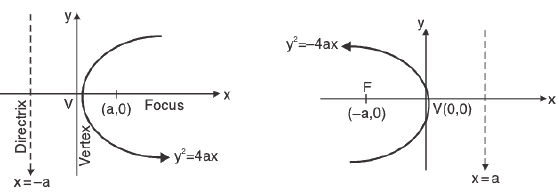
(c) Parabola:
(i) y2 = 4ax
Vertex : (0, 0)
Focus : (a, 0)
Axis : x-axis or y = 0
Directrix : x = -a
(ii)y2 = -4ax
Vertex : (0, 0
Focus : (-a, 0)
Axis : x-axis or y = 0
Directrix : a = 0
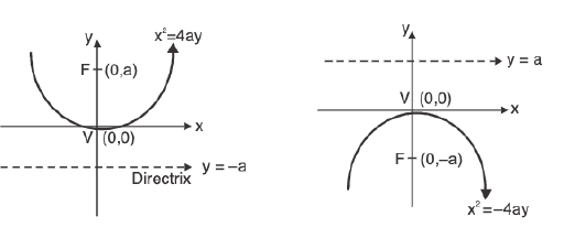
(iii) x2 = 4ay
Vertex : (0, 0
Focus : (0, a)
Axis : y-axis or x = 0
Directrix : y = -a
(iv) x2 = - 4ay
Vertex : (0, 0)
Focus : (0, -a)
Axis : y-axis or x = 0
Directrix : y = 0
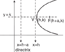
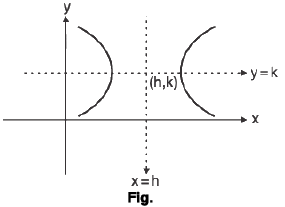
(v) (y - k)2 = 4a (x - h)
Vertex : (h, k)
Focus : (h + a, k)
Axis : x = h
Directrix : x = h - a
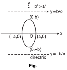
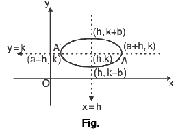
(d) Ellipse:
(i) 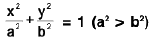
Centre : (0, 0)
Focus : (±ae, 0)
Vertex : (±a, 0)
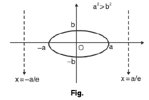
Eccentricity : e = 
Directrix : x = ± a/e
(ii) 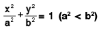
(iii)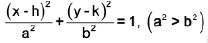
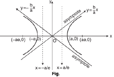
(e) Hyperbola:
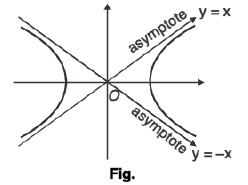
(i) 
Centre : (0, 0)
Focus : (±ae, 0)
Vertices : (±a, 0)
Eccentricity : e = 
Directrix : x = ± a/e
In above figure asymptotes are y = 
(ii)
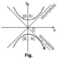
(iii) 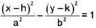
(iv) x2 - y2 = a2 (Rectangular hyperbola)
As asymptotes are perpendicular. Therefore, called rectangular hyperbola.
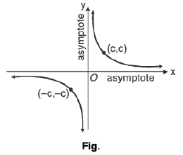
(v) xy = c2
Here, the asymptotes are x-axis and y-axis.
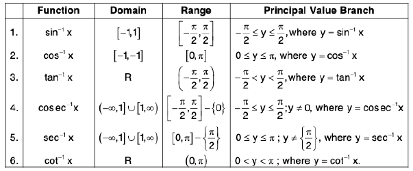
Inverse Trigonometric Curves
As we know trigonometric functions are many one in their domain, hence, they are not invertible. But their inverse can be obtained by restricting the domain so as to make invertible. Every inverse trigonometric is been converted to a function by shortening the domain.
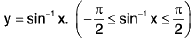
For Ex :Let f(x) = sin x
We know, sin x is not invertible for x ∈ R.
In order to get the inverse we have to define domain as:

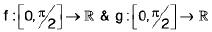
∴ If 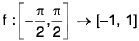 defined by f(x) = sin x is invertible and inverse can be represented by:
Similarly,
y = cos x becomes invertible when f : [0, π ] →[-1, 1]
y = tan x ; becomes invertible when 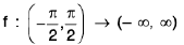
y = cot x ; becomes invertible when f : (0, π ) → [-∞, ∞]
y = sec x ; becomes invertible when 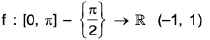
y = cosec x; becomes invertible when 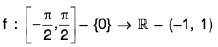
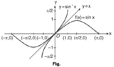
(i) Graph of y = sin-1 x ;
where,
x ∈ [-1, 1]
and y = 
As the graph of f-1(x) is mirror image of f(x) about y = x.
(ii) Graph of y = cos-1 x ;
Here,
domain ∈ [-1, 1]
Range e [0, π]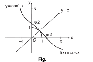
(iii) Graph of y = tan-1 x ;
Here, domain ∈ R, Range ∈ 
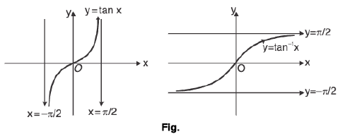
As we have discussed earlier, “graph of inverse function is image of f(x) about y = x” or “by interchanging the coordinate axes”.
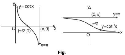
(iv) Graph of y = cot-1 x ;
We know that the function f : (0, π) → R, given by f(θ) = cot θ is invertible.
∴ Thus, domain of cot-1 x ∈ R and Range ∈ (0, π).
(v) Graph for y = sec-1 x;
The function f : 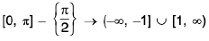 given by f(θ) = sec θ is invertible.
y = sec-1 x, has domain ∈ R - (-1, 1) and range ∈ [0, π] - π/2 : shown as
(vi) Graph for y = cosec-1 x;
As we know, f : 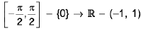 is invertible given by f(θ) = cosθ.
∴ y = cosec-1 x ; domain ∈ R - (-1, 1)
Range ∈ 
Note : If no branch of an inverse trigonometric function is mentioned, then it means the principal value branch of that function.
In case no branch of an inverse trigonometric function is mentioned, it will mean the principal value branch of that function, (i.e.,)
Bounded Function
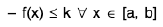
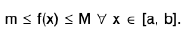
A function f : [a, b] → R is said to be bounded in the interval [a, b], if there exist two numbers k and K such that
k < f(x) < K ∀ x ∈ [a, b]. or if its range is bounded.
Thus a function is bounded in [a, b], if it is both bounded above and bounded below in [a, b].
Ex :
- f(x) = x2 is bounded in [1, 2], since 1 < f(x) < 4 ∀ x ∈ [1, 2].
- f(x) = 1/x is bounded in (0, 1).
- f(x) = x/x-1 is not bounded in [1, 4].
Results :
- Every bounded sequence has a limit points.
- A number p is a limit point of a sequence <an> iff there exists a subsequence (ank) of <an> such that ank → p.
- Every closed interval [a, b] is a closed set.
- A closed set contains all its limit points.
- If p is a limit point of a set S and S⊂T, then p is also a limit point of T.
Unbounded function
If a function is neither bounded above nor below, then this is known as an unbounded function.
Ex :
- f(x) = x is unbounded for x∈ (-∞,∞).
- f(x)= 1/x is unbounded on any interval that includes x = 0.
Properties of bounded functions
- If f,g are bounded, then f + g, f - g, f-g, and f/g are also bounded.
- If f is bounded, then I f I is bounded and also the composition fog is bounded for any function g. In particular, any transformation of f is also bounded.
- If f is bounded and g does not approach 0 arbitrarily close (that is, inf(lgl) > 0, then f /g is bounded
- A sum/difference of a bounded and an unbounded function is again unbounded.
Ex:A product of two unbounded functions may be bounded. x(1/x) = 1.
Composition of two unbounded functions may yield a bounded function.
For Ex, 1/x is unbounded, so is (ex + 1), but when we substitute the latter into the former, we get 1/(ex + 1), which is a bounded function. Indeed, inf(ex + 1) = 1, so we are separated from zero, and 1 is a bounded function (constant), so the ratio is bounded..
Limit of a Function of One Variable
If L is a real number, then limx→x0 f(x) = L means that the value f(x) can be made as close to L as we wish by taking x sufficiently close to x0. This is made precise in the following definition.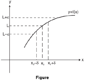
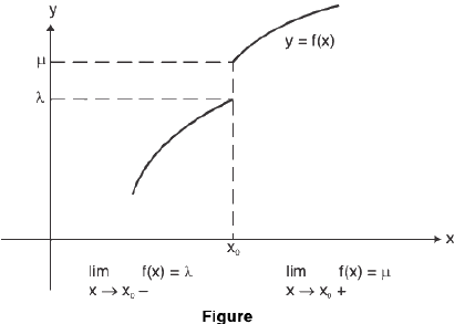
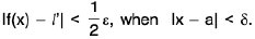
A function f is said to tend to a limit / as x tends to a, written as  if given any ε > 0 (however small), there exists some δ > 0 (depending on ε) such that I f(x) - / I < ε whenever 0 < I x - a | < δ.
Figure depicts the graph of a function for which  f(x) exists.
Solved Example
Example :  = 5
= 5
Sol: L et ε > 0 be given . We have I (2x + 3) - 5 | = | 2x - 2 | = 2 | x - 1 |.
Now I (2x + 3) - 5 | < ε when 2 I x — 1 | < ε or I x — 1 | < 1/2ε.Choosing δ = 1/2ε, I (2x + 3) - 5 | < ε when I x - 1 | < δ.
Hence
Example : If c and x are arbitrary real numbers and f(x) = cx, then 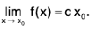
Sol: To prove this, we write lf ( x ) - c x0l = le x - c x0l = Icllx - x0l.
If c ≠0, this yields
lf(x) - cx0l < ε ------(*)
iflx - x0l < δ,
where δ is any number such that 0 < δ < ε/lcl. If c = 0, then f(x) - cx0 = 0 for all x, so (*) holds for all x.
One-Sided Limits
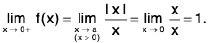
The function
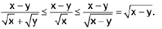
f(x) = 2x sin √x
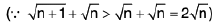
satisfies the inequality
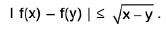
lf(x)l < ε
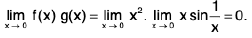
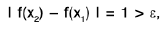
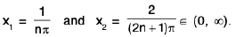
if 0 < x < δ = ε/2. However, this does not mean that limx →0 f(x) = 0, since f is not defined for negative x, as it must be to satisfy the conditions of Definition with x0 = 0 and L = 0. The function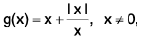
can be rewritten as
hence, every open interval containing x0 = 0 also contains points x1 and x2 such that Igf(x1) - g(x2)l is as close to 2 as we places. Therefore, limx→ xo g(x) does not exist.
Although f(x) and g(x) do not approach limits as x approaches zero, they each exhibit a definite sort of limiting behavior for all positive values of x, as does g(x) for small negative values of x. The kind of behavior we have in mind is defined precisely as follows.
Left Hand and Right Hand Limits
A function f is said to tend to a limit / as x tends to a from the left, if given any ε > 0 (however small), there exists a δ > 0 (depending on ε) such that I f(x) -/I < ε, whenever a- δ < x < a.
It is called the left hand limit at a
Remarks 1. x → a- ⇒ x → a through values less than a,
x → a+⇒ x → a through values greater than a.
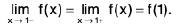
Remarks 2. Clearly,  f(x) exists if and only if
  f(x) and
  f(x) both exist and are equal.
Hence 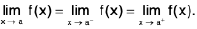
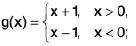
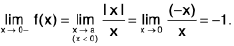
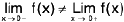
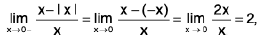
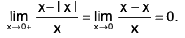
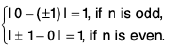
Example : I x I = x, if x ≥ 0 and I x I = - x, if x < 0
Sol:
Hence
does not exist, since
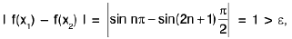
Example : Show that the function f, defined on R\{0} by f(x) = sin(1/x), whenever x ≠ 0, does not approach 0 as x → 0.
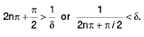
Sol: Let ε = 1/2 > 0 and let δ be any positive number.
By Archimedean property, for 1/δ > 0, ∃ π ε N such thatIf
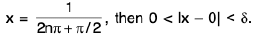
Now Isin (1/x) - 0| = |sin (2nπ + π/2) = 1 > ε.
Thus there is ansuch that for each δ > 0, ∃ some point x =
for which Isin (1/x) - 0| > ε and 0 < lx — 0| < δ .
Hence
Some Theorems on limit
Theorem : , if it exists, is unique.
Proof. Let  = l and = l' ----(1)
We shall show that / = /’. Let ε > 0 be given.
Using (1), there exists δ1 > 0 and δ2 > 0 such that ----(2)
and  ----(3)
Let δ = min (δ1, δ2). Then, by (2) and (3),
Now I/ - /’| = |/ - f(x) + f(x) - l'| 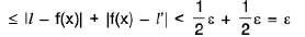
∴ I/ - / ’| < ε, when 0 < lx — a| < δ .
Since ε is arbitrarily small, I/ - /’| = 0. Hence / = /’.
Theorem : If  and
and  , then
(i) 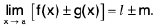
(ii) 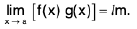
(iii)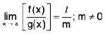
Proof.
(i) Let ε > 0 be given. There exist δ1 > 0, δ2 > 0 such that
lf(x) - /I < 1/2 ε, whenever 0 < lx - a| < δ1and lg(x) - m| < 1/2 ε, whenever 0 < lx - a| < δ2,
Let δ = min (δ1 δ2). Then
lf(x) - /I < 1/2 ε, whenever 0 < lx - a| < δ,
and lg(x) - m| < 1/2 ε, whenever 0 < lx — a| <δ,
Now lf(x) ± g(x) - (/ ± m)| = |(f(x) - /I ± (g(x) - m)|
< lf(x) - /I + lg(x) - m| < δ/2 + ε/2 = ε, when 0 < lx — a| <δ l{f(x) ± g(x)| - (/ ± m)| < δ, whenever 0 < lx - a| < δ.
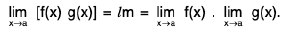
Hence lim [f(x) ± g(x)l = / ± m.
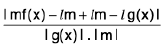
(ii) We have lf(x) g(x) - /ml
=I g(x) (f(x) - /) + /(g(x) - m) | ≤I g(x) I I f((x) - / I + I / I I g(x) - m |. ...(1)
Since
f(x) = / and
g(x) = m, for ε’ > 0, there exists some δ > 0 such that
Ig(x)- /I < ε’ and | g(x) - m | < ε' 0 <| x - a | < ε . ...(2)
Now Ig(x)I = I m + g(x) - m |≤I m I + I g(x) -m|
orIg(x) I < I m I + ε' when 0 < | x — a | < δ. ...(3)
From (1), (2) and (3) ; we obtain
I f(x) g(x) - /m I
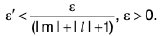
< (I m I + ε’) ε’ + | / I ε’ when 0 < | x - a | < δ
< (I m I +l / I + 1) v when 0 < | x - a | < δ. (∴ ε’ < 1)
Let us choose ε’ such that
∴ lf(x) g(x) - /ml < ε, whenever 0 < lx - a| < δ.
Hence
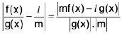
(iii) Consider=
......(1)
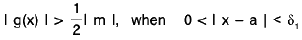
Sinceg(x) = m ≠0, so there exists a δ1 > 0 such that
⇒......(2)
Since
......(3)
Since......(4)
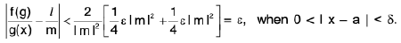
Let δ = min (δ1, δ2, δ3). From (1), (2), (3), (4) ; we get
Hence, provided m ≠ 0
Ex.Let f(x) = x2 sin (1/x), when x ≠ 0, f(0) = 0, and g(x) = x.
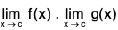
Ex. Evaluate  and
and 
Hint,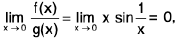
Theorem : If  , then there exists a 8 > 0 such that
Proof. Since / ≠0, so I / I > 0.
Let us choose ε > 0 such thatNow
⇒ for any ε > 0, ∃ a δ > 0 such that
lf(x) - l| < ε, when 0 < lx - a| < δ. ----(1)
Now I / 1 = I / - f(x) + f(x) | < I / - f(x) | + | f(x) |. ----(2)
From (1) and (2), I / I < ε + I f(x) I, when 0 < I x - a | < δ
⇒ I f(x) I > I / I - ε, when 0 < I x - a | < δ
⇒, hen 0 < I x - a | < δ
Hencewhen 0 < I x - a | < δ.
Theorem : Prove that
f(x) exists and is equal to a number / if and only if both left limit
f(x) and right limit
f(x) exist and are equal to /.
OR
Let f be defined on a deleted neighbourhood of c. Show that f(x) exists and equals / iff
f(c + 0), f(c - 0) both exist and are equal to /.
Proof. Condition is necessary
Let
f(x) = /. Then for any ε > 0, there exists some δ > 0 such that
lf(x)-/I <ε,when0 <lx - c| < 8
orlf(x)-/I<ε,when c - δ < x < c + δ, x ≠ c.
It follows that lf(x) -/I<ε,whenc-δ < x < c, ...(1)
and lf(x) - /I < c,whenc<x < c + δ. ...(2)
From (1) and (2), we see that
f(x) and
f(x) both exist and are equal to /.
Condition is sufficient
Let
Then for any ε > 0, there exist some δ, > 0 and δ2 > 0 such thatlf(x) - /I < ε, when c < x < c + δ1 ...(3)
and lf(x) - /I < ε, when c - δ2 < x < c. ...(4)
Let δ = min (δ1, δ2). Then 8 ≤ δ1 and δ2 ≤ δ2⇒ c + δ ≤ c + δ1 and c - δ ≥ c - δ2 (or c - δ2 < c - δ). ...(5)
From (3), and (5), we obtainlf(x) - /I < ε, when c < x < c +δ1
and lf(x) - /I < ε, when c - δ < x < c.If(x) — /I < ε, when c - δ < x < c + δ1 x ≠ c
orlf(x) — /I < ε, when 0 < lx - c| < δ.
Hencef(x) = /.
Ex : Show that  does not exist.
We have
andL.H.L ≠ R.H.L
Hence
Infinite Limits or Limits at Infinity
Definition :The expression  f(x) = / means, given any ε > 0, there exists some M > 0 such thatI f(x) - l I < ε, when x > M.
Definition :The expression  means, given any M > 0 (however large), there exists some δ > 0 such that
f (x) > m, whenever I x - a | < δ.
Definition :The expression  means, given any M > 0 (however large), there exists some δ > 0 such that
f(x) < -M, whenever I x - a | < δ.
Ex : Show that
(i) 
(ii) 
(iii) 
(i)Let M > 0 be any large number. Let δ = 1/M.
Then 0 < x < δ ⇒ 
Hence  by
by
(ii)Again - d < x < 0 ⇒  ⇒
⇒  ⇒
⇒ 
Hence  by
by
Note :  does not exist.
(iii)Now - δ < x < δ ⇒  ⇒
⇒ 
Hence  by
by
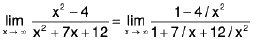
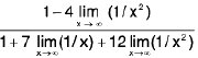
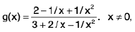
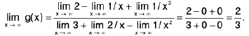
Example: Find 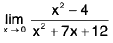
Sol: Dividing numerator and denominator by x2, we get
=
=
= 1

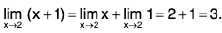
Example: Find  and
and 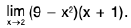
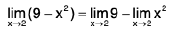
Sol: If c is a constant, then
c = c, and, from Example
x = x0,. Therefore, from Theorem
=
= 9 - 22 = 5,
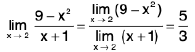
and
Therefore,
and


Example :Let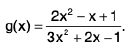
Sol: it leads to an indeterminate form as x tends to infinity. Rewriting it as
we find that
Monotonic Functions
A function f is non-decreasing on an interval I if
f(x1) < f(x2) whenever x1 and x2 are in I and x1 < x2, ...(1)
Similarly, A function f is non-increasing on I if
f(x1) > f(x2) whenever x1 and x2 are in I and x1 < x2. ...(2)
In either case, f is monotonic on I. If < is replaced by < in (1), f is said to be strictly increasing on I. If > is replaced by > in (2), f is said to be strictly decreasing on I. In either of these two cases, f is strictly monotonic on I.
Ex :The function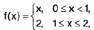 is non-decreasing on I = [0, 2] and - f is non-increasing on I = [0, 2].
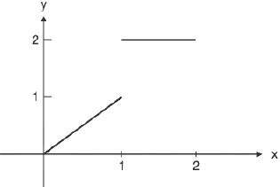
The function g(x) = x2 is increasing on [0, ∞) Figure,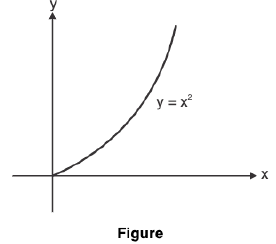
and h(x) = -x3 is decreasing on (-∞, ∞) Figure.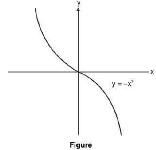
Properties of Monotonic Functions
- If f is monotonic then, for any monotonic sequence <an>, <f(an)> is also monotonic.
- Sum of two monotonically increasing (decreasing) sequence again monotonically increasing (decreasing).
- Difference of two monotonically increasing (decreasing) sequence may not be monotonically increasing (decreasing).
Ex :
such that f(x) = sinx & g(x) = x
but (f - g)(x) = sinx - x is not monotonic.
(iv) Similarly product of two monotonically increasing (decreasing) sequences may not be monotonically increasing (decreasing).
Ex: f: R→ M & g : R → R
such that f(x) = x & g(x) = x
but (fg)(x) = x2 is not monotonic.
(v)If the function f is increasing (decreasing), then the inverse function 1/f is decreasing (increasing).(vi) Composition of two monotonic functions f:X →Y & g : Y →Z is monotonic g of: X→ Z.
Continuous Functions of One Variable
Consider a function f : [a, b] → R, Let a < c < b i.e. c ∈[a,b].
Definition : A function f is said to be continuous at a point c, if for any ε > 0, there exist some δ > 0 such that
I f(x) - f(c) | < ε, whenever I x - c | < δ ...(1)
or 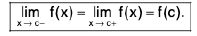
A function f is said to be continuous in an interval [a, b], if it is continuous at every point of the interval [a, b].
Remark : If a function f is not continuous at a point c, then from (1), it follows that there exists some ε > 0 such that for each δ > 0, there is some y ∈ [a, b] satisfying
| f(y) - f(c) | > e, when I y - c | < δ.
Definition :A function f is said to be discontinuous at a point x = c, if f is not continuous at
x = c.
Remark :The discontinuity of a function f at x = c is obtained in either of the following cases:
- f is not defined at x = c.
 f(x) does not exist.
 f(x) exists but
  f(x) ≠ f(c).
Algebra of Continuous Functions
- The identity function f(x) = x is continuous in its domain.
- If f(x)and g(x) are bothcontinuous at x =c,so is f(x) + g(x)at x= c.
- If f(x) and g(x) are both continuous at x =c,so is f(x) * g(x) at x = c.
- If f(x) and g(x) are both continuous at x =c,and g(x) * 0, then f(x) / g(x) is continuous
- at x = c.
- If f(x) is continuous at x = c, and g(x) is continuous at x = f(c), then the composition g(f(x)) is continuous at x = c
Solved Example
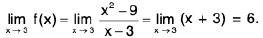
Example 1: The function defined as 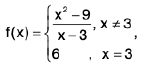 is continuous at x = 3.
Sol: We have
Since f(3) = 6,
Hence f is continuous at x = 3.

Example 2: Show that the function 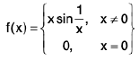 is continuous at x = 0.
Sol: We know
{Since sin(1/x) is bounded}
Also f(0) = 0.So
Hence f is continuous at x = 0.
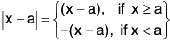
Example 3: Show that 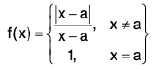 is discontinuous at x = a.
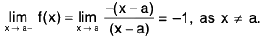
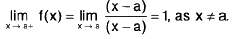
Sol: We know
Now
Thusdoes not exist and so f is discontinuous at x = a.
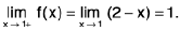
Example 4: Examine the continuity of the function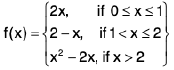 at x = 1 and x = 2.
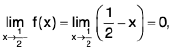
Sol: We have
=
2x = 2
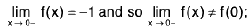
Thusf(x) does not exist and so f is discontinuous at x = 1.
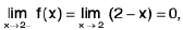
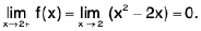
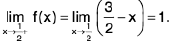
Now
Also f(2 ) = 2 - 2 = 0.
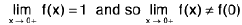
Thusf(x) =
f(x) = f(2) and so f is continuous at x = 2.
Example 5: Show that the function 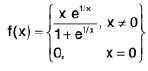 is continuous at x = 0.
Sol: We have
∴(∴f(0) = 0)
Hence f is continuous at x = 0.
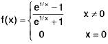
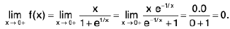
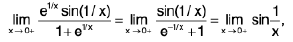
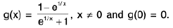
Example 6: Show that the function 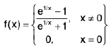 is discontinuous at x = 0.
Sol:
By computing two sided limit
Left Hand Limit (LHL)
=
Right Hand Limit (RHL)
=
=
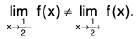
RHL ≠ LHL ≠ f(0)
So f is discontinuous at x = 0.
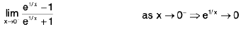

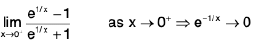
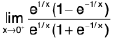
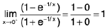
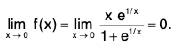
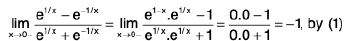
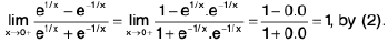
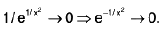
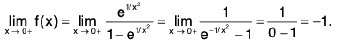
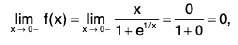
Example 7: Show that the function 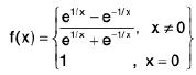 is discontinuous at x = 0.
Sol: We know x → 0- ⇒ e1/x → 0 ...(1)
and x → 0+ ⇒ e-1/x → 0 ...(2)
∴
Hencedoes not exist (∴ -1 ≠ 1)
and so the given function is discontinuous at x = 0.
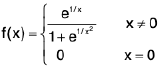
Example 8: Examine the continuity of the function : 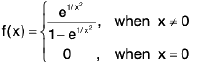 at x = 0.
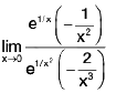
Sol: Clearly, x → 0+ ⇒ 1/x2 -> + ∞ ⇒ e1/x2 → + ∞
⇒
Similarly,
Hence f is discontinuous at x = 0.

Example 9: Show that the function f defined on R by setting 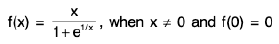 is continuous at x = 0.
Sol:
Also f(0) = 0. Hence f is continuous at x = 0.
Example 10: Show that f(x) = I x I + I x - 1 | is continuous at x = 0 and x = 1.
Sol: f(x) = - x - (x - 1) = 1 - 2x, when x < 0; . . . (1)
f(x) = x - (x - 1) = 1 when 0 < x < 1 ; . . . (2)
Nowby (2).
Also f(0) = I 0 I + I 0 - 1 | = 1.
∴
Hence f is continuous at x = 0.
Nowby (2).
by (3).
Also f(1) = I 1 I + I 1 - 1 | = 1.
∴
Hence f is continuous at x = 1.
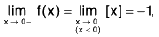
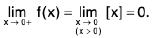
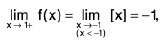
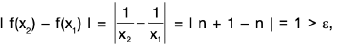
Example 11: Let f be the function defined on R by setting f(x) = [x], for all x ∈ R, where [x] denotes the greatest integer not exceeding x. Show that f is discontinuous at the points x = 0, ± 1, ± 2, ± 3, ... and is continuous at every other point.
Sol: By definition, we have
[x] = 0, for 0 ≤ x < 1,
[x] = 1, for 1 ≤ x < 2,
[x] = 2, for 2 ≤ x < 3,
[x] = -1, for -1 ≤ x < 0.
[x] = -2 for -2 ≤ x - 1 and so on.
At x = 0
Since, f is discontinuous at 0.
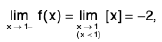
At x = 1
So f is discontinuous at -1.Similarly, f is discontinuous at - 2, - 3, - 4, ...
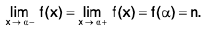
Let α ∈ R - Z be any real number but not an integer. Then there exists an integer n such that n ≤ α < n + 1. Then
[x] = n, for n ≤ x < n + 1.
Now
Hence f is continuous at α.
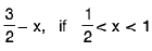
Example 12: Let f be the function on [0, 1] defined by 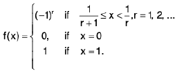 Examine the continuity of f at 1, 1/2 ,1/3 ...
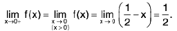
Sol: We observe that
(r = 1)
= 1, If(r = 2)
= -1, if(r = 3)
and so on.
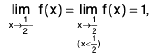
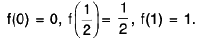
At x = 1.= 1
Sincef is continuous at x = 1.
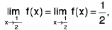
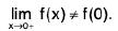
At x = 1/2
Thus f is discontinuous at 1/2
Similarly, f is discontinuous at 1/3, 1/4, 1/5...
Example 13: Show that the function f on [0, 1] defined as  when
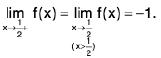
when 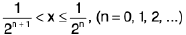 is discontinuous at
  ,.....
Sol: We observe that
f(x) = 1 when 1/2 < x ≤ 1 (n = 0 )
= 1/2 when 1/22 < x ≤ 1/2 (n = 1 )
= 1/22 when 1/23 < x ≤ 1/22 (n = 2) and so on.
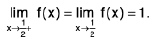
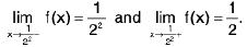
At x = 1/2
Thus f is discontinuous at x = 1/2
At x = (1/2)2
Thus f is discontinuous at x = (1/2)2 and so on.
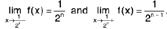
At x = (1/2)n
Hence f is discontinuous at (1/2)n , n = 1, 2, ...
Example 14: Let f be a function defined by : 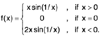 Discuss the continuous of f at x = 0.
Sol: We see that
= 0,
Also f(0) = 0.
Hence f is continuous at x = 0.
Example 15: Examine the continuity of the function : f(x) = 2x - [x] + sin (1/x), x ≠ 0 ; f(0) = 0 at x = 0 and x = 2, where [x] denotes the greatest integer not greater than x.
Sol: By Example
and
do not exist.
Alsodoes not exist.
Thusf(x) and
f(x) do not exist and so the given function is discontinuous at x = 0, 2.
Example 16: Let f be the function defined on R by setting 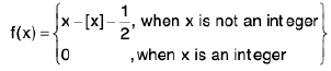 Show that f is continuous at all points of R ~ Z and is discontinuous whenever x ∈ Z.
Sol: Let n ∈Z = {0, ± 1, ± 2, ± 3, ...} be arbitrary.
Thendoes not exist and so
does not exist.
Hence f is discontinuous whenever n ∈ Z.We observe that
[x] = 0, if 0 ≤ x < 1,
[x] = 1, if 1 ≤ x < 2,
[x] = 2, if 2 ≤ x < 3,
.............................
[x] = m, if m ≤ x ≤ m + 1 and so on.
Using these, we obtain
f(x) = 1/2 if 0 ≤ x < 1,
f(x) = x - 1 - 1/2 = x - 3/2, if 1 ≤ x < 2,
f(x) = x -2 - 1/2 = x - 5/2, if 2 ≤ x < 3 and so on.
he above relations are all linear and so f is continuous at all positive non-integral points. Similarly, f is continuous at all negative non-integral points, sinceif - 1 ≤ x < 0
=if - 2 ≤ x < - 1 etc.
Hence f is continuous at all points of R ~ Z.
Types of Discontinuities
- The function f is said to have a removable discontinuity at x = c, if
 exists but is not equal to f(c). If we redefine f(c), then f will become continuous.
 - If is said to have a discontinuity of the first kind at x = c, if
 and
and  both exist but are not equal.
 - If is said to have a discontinuity of the first kind from the left at x = c, if
 exists but is not equal to f(c).
 - If is said to have a discontinuity of the first kind from the right at x = c, if
 exists but is not equal to f(c).
 - If is said to have a discontinuity of the second kind from the left [right] at x = c, if

 does not exist.
Solved Example
Example 1: The function f(x) =  and f(0) = 1 has a removable discontinuity at the origin.
Sol: We have
Also f(0) = 1, ∴
Hence f has a removable discontinuity at x = 0.
Example 2: Examine the continuity of the function f defined by 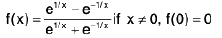 at x = 0. Also discuss the kind of discontinuity if any.
Sol: We have,
Hence f has a discontinuity of the first kind from the left and the right at x = 0.
Example 3: A function f is defined by 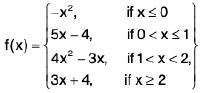 Examine f for continuity at x = 0, 1,2. Also discuss the kind of discontinuity, if any.
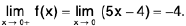
Sol: At x = 0.
Also f(0) = 0.
Thusand so f has a discontinuity of the first kind from the right at x = 0.
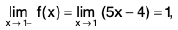
At x = 1.
and f(1) = 5 x 1 - 4 = 1.
Thusand so f is continuous at x = 1.
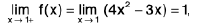
At x = 2.= 4 x 4 - 3 x 2 = 10,
= 10
Also f(2) = 3 x 2 + 4 = 10.
Thusand so f is continuous at x = 2.
Example 4: Obtain the points of discontinuity of the function f defined on [0, 1] as follows : 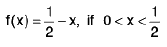 =
= 
 Also examine the kind of discontinuities.
Sol: At x = 0.
Also f(0) = 0. ∴
Thus f has a discontinuity of the first kind from the right at 0.
At x = 1/2
∴
Thus f has a discontinuity of the first kind at x = 1/2
At x = 1.= 1/2. Also f(1) = 1.
∴
Thus f has a discontinuity of the first kind from the left at x = 1.

Example 5: Examine for continuity at x = 0, the function 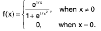
Sol:
By applying L-Hospital rule-
=
=
= 0⇒ f is continuous at x = 0.


Example 6: Examine the function 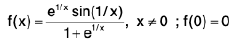 for points of discontinuity, if any.
Sol: We know that
x → 0- ⇒ e 1/x → 0 and x → 0 + ⇒ e-1/x → 0.
∴
which does not exist. Hence f has a discontinuity of the second kind from the right at x = 0.
Theorems on Continuous Functions
Theorem : (a) If two functions f, g are continuous at a point c, then the functions f + g, f - g, fg are also continuous at c and if g (c) ≠ 0, then f / g is also continuous at c.
(b) Prove that if a function f is continuous at x = a, then I f I is also continuous at x = a. But the converse if not true
Proof. Since f and g are continuous at c,
---(1)
We show that f + g is continuous at c. We have
=
∴
Thus f + g is continuous at c.
Again,
=
= f(c) g(c) = (fg) (c).
Thus fg is continuous at c
Similarly, we can prove the remaining parts.
(b) Since f is continuous at x = a, therefore, for ε > 0 there exists some δ > 0 such that
I f(x) - f(a) | < ε when 0 < I x - a | < δ ...(2)
We know l l x l - | y | | ≤ l x — y | ∀ x, y ∈ R.
∴ I I f(x) I - | f(a) | | < I f(x) - f(a) | < ε, 0 < I x — a | < δ, using (2)
Hence I f I is continuous at x = a.However, if I f I is continuous at x = a, then f may not be continuous at x = a as seen below:
Let
Then I f(x) | = 1 ∀ x ∈ R and so I f I is continuous at every point of R, but f is discontinuous at every point of R.
Remarks : 1. Let f and g be defined on an interval I. If f + g and fg are continuous at a point p ∈ l , then f and g may not be continuous at p as explained by the following examples :
(i) Let 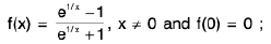
Thus f and g are discontinuous at x = 0, but f + g = 0 (being a constant function) is continuous at x = 0.
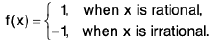
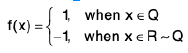
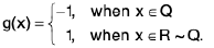
(ii) Let f(x) = g(x) = 1, when x is rational
f(x) = g(x) = - 1 , when x is irrational.
By Example, f and g are discontinuous at every point of R, but fg = 1 (being a constant function) is continuous at every point of R.
Similarly, we can give examples to show that if f - g, f/g are continuous at a point p ∈ I; then f and g may not be continuous at p.
Notice that in (ii), f/g = 1 ∀ x ∈ R ⇒ f/g continuous ∀ x ∈ R.
If in (i), g(x) = f(x), then f - g = 0 ⇒ f - g is continuous ∀ x ∈ R.
2. A polynomial function f(x) = a0 + a1x + a2x2 + ... + anxn is continuous for all x ∈ R.
Clearly  = cn ∀ n ∈ N ⇒ xn is continuous ∀ x ∈ R, ∀ n ∈ N.
Also an (being a constant) is continuous. By Theorem , anxn is continuous ∀ n ∈ N and ∀ x ∈ R. Hence a0 + a1x + a2x2 + ... + anxn is continuous ∀ x ∈ R.
Theorem : A function f defined on an interval I is continuous at a point p ∈ I if and only if for each sequence <pn) converging to p, the sequence <f(pn)> converges to f(p).
Proof. The condition is necessary.
We are given that the function f is continuous at p and the sequence <pn> converges to p. We shall show that <f(pn)> converges to f(p). Since f is continuous at x = p, therefore for ε > 0, there exists a δ > 0 such that
I f(x) - f(p) | < ε, when I x - p | < δ. ...(1)
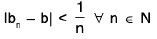
Since the sequence (pn> converges to p, so there exists some positive integer m such that
lpn - p| < δ ∀ n ≥ m. ...(2)
Replacing x by pn in (1), we get
I f(Pn) - f(P) I < ε when I pn - p | < δ. ...(3)
From (2) and (3), we obtain I f(Pn) - f(P) I < ε ∀ n ≥ m. Thus <f(pn) - f(p).
The conditions is sufficient.Let <pn) → p ⇒ <f(pn)> → f(p).
We shall show that f is continuous at x = p.Let, if possible, f be not continuous at x = p.
Then for some ε > 0 and for each δ > 0, E at least one x such that
I f(x) - f(p) | ≥ ε, whenever I x - p | < δ.
Let δ = 1/n. Then ∀ n ∈ N, there exists x = pn such that
I pn - p | < 1/n ⇒ I f(pn) - f(p) | ≥ ε
i.e.,
Thus we have proved that there is a sequence <pn) such that (pn> converges to p, but the sequence <f(pn)> does not converge to f(p). This is a contradiction to the given condition. Hence f is continuous at x = p.

Theorem : Let f be a function defined on an interval I and p ∈ I. Let g be a function defined on an interval J such that f(l) ⊆ J. If f is continuous at p and g is continuous at f(p), then show that g of is continuous at p.
Proof. Let (pn be any sequence in I such that pn → p. ...(1)
Since f is continuous at p, so by Theorem, f(pn) → f(p).
Since f(l) ⊆ J, so <f(pn)> is a sequence in J converging to f(p) ∈ J.
Since g is continuous at f(p) and f(pn) → f(p) in J, so
g(f(pn)) → g(f(p))or(gof) (pn) -> (gof) (p). ...(2)
[By definition, (gof) (x) = g (f(x)) ∀ x ∈ I.]
From (1) and (2), it follows that gof is continuous at p
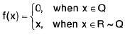
Example: F be a function on R defined by 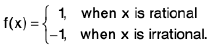 f is discontinuous at every point of R
Hint.Since Q, R-Q are dense in R , therefore for every a e R we can always find sequences from Q & R-Q that converge to a.
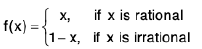
Example: Show that the function f defined by 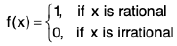 is discontinuous at every point.
Sol: Case I. Let a be any rational number so that f(a) = 1.
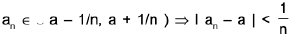
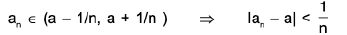
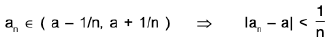
Then any nbd. (a - 1/n, a + 1/n ) of a contains an irrational number an for each n ∈ N i.e.,
⇒ lan - a | → 0 as n → ∞ <an> → a.
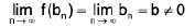
Now f(an) = 0 ∀ n (∴ an is irrational) and f(a) = 1
⇒does not converge to f(a).
Thus f is discontinuous at all rational points.
Case II.Let b be any irrational number so that f(b) = 0.
As argued earlier, we can choose a rational number bn such that
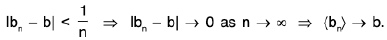
⇒ lbn - b| → 0 as n → ∞ ⇒ (bn> → b.
Now f(bn) = 1 ∀ n (∴ bn is rational) and f(b) = 0
⇒oes not converge to f(b).
Thus f is continuous at all irrational points.
Hence the given function is discontinuous at every point of R.
Example: Show that the function f defined on R by 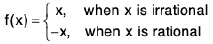 is continuous only at x = 0.
Sol: Case I : Let a ≠ 0 be any rational number so that
f(a) = - a.
Then any nbd. ( a - 1/n, a + 1/n ) of a contains an irrational number an for each n ∈ N i.e.,
Now f(an) = an ∀ n ( ∴ an irrational)
⇒
⇒ <f(an)> does not converge to f(a), when (an) → a.
So f is discontinuous at all non-zero rational points.
Case II.Let b ≠ 0 be any irrational number so that f(b) = b.As argued earlier, there exists a rational number bn ∀ n ∈ N such that
Now f(bn) = bn ∀ n (∴ bn is rational)
⇒
⇒ <f(bn)> does not converge to f(b). (∴ f(b) = 0)
Thus f is discontinuous at every non-zero irrational point.
Now we shall prove that f is continuous at x = 0.
We have f(0) = 0 and
lf(x) - f(0)| = |f(x)| = |x|, if x is rational = 0, if x is irrational
Let ε > 0. Then I f(x) - f(0) | < ε, for I x - 0 | < δ (δ = ε).Hence f is continuous only at x = 0.
NOTE: we can also use sequential approach to deal with such questions on which f(x) is defined explicitly on all rationals & irrationals. It will consume time in exam.
As let a ε RThen there exist <an > ε Q such that <an > → a
Similarly, there exist <bn> ε R - Q such that <bn> → a
now to find points of continuity we first look for the points where limit exist
for that lim <f(an)> = lim <f(bn)> ⇒ a = -a ⇒ a=0.
It is the only point where continuity is to be checked.
since 0 ε Q ⇒ f(0)=0 = lim <f(an)>=lim <f(bn)> ∀ <an> ε Q such that <an> → 0 ∀ <bn> ε R-Q such that <bn>→ 0.
Hence f is continuous only at x = 0.


Example: Let f be a function defined on (0, 1) by : 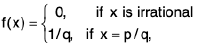 where p and q are positive integers having no common factor. Prove that f is continuous at each irrational point and discontinuous at each rational point.
Sol: Case I.Let a ∈ (0, 1) be any rational number so that a = p/q, where p and q are positive integers having no common factor. Then f(a) = 1/q (as given).
Any nbd. ( a - 1/n, a + 1/n ) of a contains an irrational number an, for each n ∈ N i.e.,
⇒ lan - a| → 0 as n - » ∞ ⇒ <an) → a.
Now f(an) = 0 ∀ n (∴ an is irrational)
⇒ <f(an)> → 0 ≠ f( a ) ( ∴ f( a ) = 1 /q > 0.]
Hence f is discontinuous at every rational point in ( 0, 1 ).
Case II. Let b ∈ ( 0, 1 ) be any irrational number, so that
f(b) = 0
Let ε > 0 be given. We can choose a positive integer n such that
1/n < ε.
It is clear that there an can be only a finite number of rational numbers p/q in (0, 1) such that q < n.
We can, therefore, find some δ > 0 such that no rational number //m in (δ - 5, δ + 5) has its denominator less than n i.e., m ≥ n.
Thus I x - b | < δ ⇒ I f(x) - f(b) | = | f(x) - 0 | = 0 < ε, ...(1)
if x is irrational.
If x = //m is rational such that I x - b | < δ, then
I x - b | < δ ⇒ I f(x) - f(b) = | f(x) | < 1/m < 1/n < ε. ( ∴m ≥ n) ...(2)
From (1) and (2), we have
I x - b | < δ ⇒ I f(x) - f(b) | < ε.
Hence f is continuous at every irrational point b in (0, 1).
Example: Show that the function f defined as 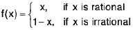 is continuous only at x = 1/2.
Sol: Case I. Let a ≠ 1/2 be any rational number. Then f(a) = a.
We can find an irrational number an for each n ∈ N such that
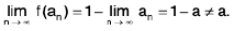
Now f(an) = 1 - an ∀ n (∴ an is irrational)
⇒
(Observe that if a = 1/2, then 1 - a = a).
⇒ <f(an)> does not converge to f(a). (∴ f(a) = a)
Thus f is discontinuous at all rational points a ≠ 1/2
Now we shall show that f is continuous at x = 1/2 only.
We haveif x is rational
=if x is irrational.
Thus
Let ε > 0 be given. Choose δ = ε > 0. Thenwhen
Hence f is continuous only at 1/2.


Example: Let f satisfy f(x + y) = f(x) + f(y) ∀ x, y ∈ R . ...(1)
Show that if f is continuous at a point c, then f is continuous at all points of R.
Sol: (i) Taking x = y = 0 in (1), we obtain
f(0) = f(0) + f(0) ⇒ f(0) = 0. ..(2)
Taking y = - x in (1), we obtain
f(0) = f(x) + f(- x) ⇒ 0 = f(x) + f(- x), using (2)
f(- x) = - f(x) ∀ x ∈ R. ...(3)
Let (cn) be any sequence of real numbers such that cn → 0.
Then cn + c → 0 + c = c⇒ f(cn + c) → f(c), as f is continuous
⇒ f(cn) + f(c)→ f(c), using (1)
=⇒ f(cn) → 0.
Thus cn →0 ⇒ f(cn) → 0.
Let x be any real number. We shall show that f is continuous at x. Let <xn> be a sequence of real numbers such that xn → x
⇒xn - x → 0
⇒ f(xn - x) → 0, using (4)
⇒ f(xn) + (-x) → 0, using (1)
⇒ f(xn) - f(x) → 0, using (3)
⇒f(xn) → f(x).
Since xn → x ⇒ f(xn) → f(x), f is continuous for all x ∈ R.
Example: Prove that the function h(x) = √sinx is continuous on [0, π].
Sol: First of all, we show that f(x) = √x is continuous ∀ x ≥ 0.
Let c > 0 so that f(c) = √c . For x ≥ 0, we have
Let ε > 0 be given. Then
If(c) - f(c)| < ε, whenever lx - c| < δ, δ = √c ε > 0.
Hence f is continuous at c > 0.
Obviously,. Hence f is continuous for all x ≥ 0.
Next we show that g(x) = sin x is continuous for all x I R.
For c ∈ R, we have
= lx - c|,
Let ε > 0 be given. Then lg(x) - g(c)| < ε for lx - c| < δ, δ = ε > 0.Hence g is continuous for all c ∈ R.
It is clear that h = fog, where g(x) = sin x, x ∈ [0, π] and f(x) = √x, x ≥ 0. By Theorem h(x) = √sinx is continuous on [0, π].
Example: Given examples of two discontinuous functions f and g such that
(i) fog is continuous but gof is not continuous.
(ii) fog and gof are both continuous.
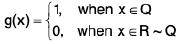
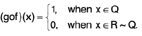
Sol: (i) We define two functions f and g as follows :
and
Then f is discontinuous at each non-zero point of R and g is discontinuous at each of R
If x ∈ Q, then (fog) (x) = f(g(x)) = f(1) = 0.If x ∈ R ~ Q, then (fog) (x) = f(g(x)) = f(0) = 0.
∴ (fog) (x) = 0 ∀ x ∈ R. Hence fog is continuous ∀ x ∈ R.
If X ∈ Q, then (got) (x) = g (f(x)) = g(0) = 1.If x ∈ R ~ Q, then (qof) (x) = q (f(x)) = q(0) = 0.
Thus
By Example gof is discontinuous ∀ x ∈ R.
(ii) We define two functions f and g on R as follow :
and
Thus f and g are discontinuous at all points of R.
If x ∈ Q, then (fog) (x) = f(g(x)) = f(—1) = 1. (∴ -1 ∈ Q)If x ∈ R ~ Q then (fog) (x) = f(g(x)) = f(1) = 1. (∴ 1 ∈ Q)
⇒ (fog) (x) = 1 ∀ x ∈ R ⇒ fog is a constant function on R.
It may be noticed that (gof) (x) = -1 ∀ x ∈ R and so gof is continuous at all points of R.
Theorem :If a function f is continuous on a closed bounded interval [a, b], then it is bounded in [a, b].
Proof. Let, if possible, f be not bounded above in [a, b].
Then for each positive integer n, we can find a point xn e [a, b], such that
f(xn) > n ∀ n ∈ N. ----(1)
Since xn ∈ [a, b] for each n ∈ N, a < xn ≤ b ∀ n ∈ N.
Thus <xn> is a bounded sequence and so it must have a limit point say p (Bolzano-Weierstrass Theorem).
Obviously, p is a limit point of [a, b]. [Result (e)]
Now [a, b] being a closed interval is a closed set and so p ∈ [a, b].
Since p is a limit point of the sequence <xn>, therefore, there exists a subsequence (xnk} of axnh such that xnk → p. ----(2)
From (1), f (xnk) > nk for all k ⇒ < f(xnk) > diverges to ∞
⇒ f (xnk) does not converge to f(p). ----(3)
From (2) and (3), it follows that f is not continuous at the point p ∈ [a, b]
This is contrary to the hypothesis that f is continuous at every point of [a, b]. Hence f is bounded above on [a, b].
Now we show that f is bounded below on [a, b].
Since f is continuous in [a, b], - f is also continuous in [a, b] and so - f is bounded above . Consequently, there exists some k ∈ R such that
⇒
⇒ f is bounded below in [a, b].
Hence f is bounded in [a, b].

Theorem : If a function f is continuous an a closed bounded interval [a, b], then it attains its bounds in [a, b]
Proof. Since f is continuous in [a, b], therefore, it is bounded in [a, b]. Let M = sup f and m = inf f.
∴
We shall show that there exist points α, β ∈ [a, b] such that
f(α) = M and f(β) = m.
We shall prove it by contradiction.
Let f(x) ≠ M ∀ x ∈ [a, b]
⇒ M - f(x) ≠ 0, ∀ x ∈ [a, b].
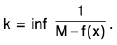
Since f is given to be continuous in [a, b] and M, being a constant function, is also continuous in [a, b], therefore M - f(x) is continuous in [a, b]. Since M - f(x) ≠ 0, ∀ x ∈ [a, b], thereforeis continuous in [a, b].
⇒is bounded in [a , b]
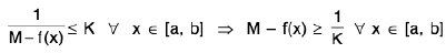
Letand k =
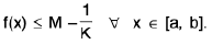
⇒
⇒
⇒
is an upper bound of f, which contradicts the fact that M is the l.u.b. of f.
Hence there exists some a α ∈ [a, b] such that f(α) = M.Similarly, there exists some β ∈ [a, b] such that f(β) = m.
Remark: If a function is not continuous on a closed interval, then it may not attain its bounds as shown below :
1. The function f(x) = x∀ x ∈ [0, 1) is continuous and bounded in [0, 1), 0 ≤ f(x) < 1 ∀ x ∈ [0, 1) ; inf f = 0 and sup f = 1. Here inf f is attained but sup f is not attained, since there is no point of [0, 1) at which f(x) = 1. (Observe that the domain of f is not a closed interval)
2. The function f(x) = x ∀ x ∈ (0, 1] is continuous and bounded in (0, 1], attains the supremum 1 and does not attain the infimum 0.
3.The function f(x) = x ∀ x ∈ (0, 1) is continuous and bounded in (0, 1), but attains neither the supremum 1 nor the infimum 0.
4. The function f(x) =1/x ∀ x ∈ (0, 1]. Here f attains the supremum 1 and does not attain the infimum 0.
Ex. Prove that if f is continuous in [a, b] and c is the infimum of f in [a, b], then there exists an x0 in [a, b] such that f(x0) = c.
Proof . We have c = int f in [a, b] i.e., c ≤ f(x) ∀ x ∈ [a, b].
Let, if possible, f(x) ≠ c ∀ x ∈ [a, b]. It follows thatis continuous in [a, b]
⇒is bounded above in [a, b]
⇒k being some real number
⇒
⇒ c + (1/k) is a lower bound of f in [a, b], where c + (1/k) > c.
The contradicts the given condition c = inf f. Hence there exists some x0 ∈ [a, b] such that f(x0) = c.

Theorem : If a function f is continuous in [a, b] and c ∈ (a, b) such that f (c) ≠ 0, then there exists some δ > 0 such that f(x) has the same sign as f(c) for all x ∈ ( c - δ, c + δ).
Proof. Since f is continuous at c, for any ε > 0, ∃ some δ > 0, such that
I f(x) - f(c) | < c, when lx — c| < δ .
i.e., f(c) - ε < f(x) < f(c) + c, when c - δ < x < c + δ. ...(1)
Case I. Let f(c) > 0. We choose ε > 0 such that
ε < f(c) ⇒ f(c) - ε > 0. ...(2)
From (1) and (2), f(x) > f(c) - ε > 0, when x ∈ ( c - δ, c + δ ).
Case II.Let f(c) < 0 ⇒ f(c) > 0. We choose ε > 0 such that
ε < - f(c) ⇒ f(c) + ε < 0. ...(3)
From (1) and (3), f(x) < f(c) + ε < 0, when x ∈ ( c - δ , c + δ ) .
Hence f(x) has the same sign as f(c) ∀ x ∈ (c - δ, c +δ).
Corollary, (i) If a function f is continuous at x = a and f(a) ≠ 0, then there exists some δ > 0, such that f(x) has the same sign as f(a) ∀ x ∈ [a, a + δ).
(ii)If a function f is continuous at x = b and f(b) ≠ 0, then there exists some δ > 0, such that f(x) has the same sign as f(b) ∀ x ∈ ( b - δ, b ].
Theorem : If a function f is continuous in [a, b] and f(a) and f(b) are of opposite signs, then there exists some point c ∈ ( a, b ) such that
f(c) = 0.
Proof. Since f(a) and f(b) are of opposite signs, we may take
f(a) > 0 and f(b) < 0.
Let S be a subset of [a, b] defined as follows :
S = {x : a ≤ x ≤ b and f(x) > 0}. ...(1)
Then S is non-empty [ ∴ f(a) > 0 ⇒ a ∈ S]
and S is bounded above with b as its upper bound.
By order-completeness property of R, S has the supremum.
Let c = sup S , c ∈ [a, b].
Now we shall prove that c ≠ a and c ≠ b, so that c ∈ ( a, b ).
Since f is continuous at x = a and f(a) > 0, ∃ a δ1 > 0 such that
f(x) < 0 ∀ x ∈ (b - δ2 b], [by corollary of Theorem] ...(2)
⇒ b - δ2 is an upper bound of S, for otherwise, there exists some y ∈ S such that y > b -δ2
i.e., b - δ2 < y ≤ b ⇒ f(y) < 0, by (2). ...(3)
As y ∈ S, f(y) > 0, by (1). This contradicts (3).
Since c = sup S, so c ≤ b - δ2 ⇒ c ≠ b.
Thus c ≠ a and c ≠ b ⇒ c ∈ (a, b).
Finally, we show that f(c) = 0.Case I. Let f(c) > 0
Since f is continuous at c and f(c) > 0, so ∃ a δ3 > 0 such that
f(x) > 0 ∀ x ∈ ( c - δ3, c + δ3). ...(4)
Let α be a number such that c < α < c + δ3. ...(5)
∴ α ∈ ( c, c + δ3) ⇒ f(α ) > 0, by (4) ⇒ α ∈ S, by (1).
∴ α < c (∴ c = sup S) or c ≥ α, which contradicts (5).
Thus f(c) ≥ 0.Case II. Let f(c) < 0.
Since f is continuous at x = c and f(c) < 0, so ∃ a δ4 > 0 such that
f(x) < 0 ∀ x ∈ ( c - δ4, c + δ4) ...(6)
Now c = sup S ⇒ ∃ at least one β ∈ S such that c - δ4 < β ≤ c
⇒β ∈ ( c - δ4, c] ⇒ f(p) < 0, by (6).But β ∈ S ⇒ f(β) > 0, which
f(c) ≤ 0. Also f(c)≥ 0.
Hence f(c) = 0 for some c ∈ ( a, b ).
Theorem by (Inverse Function Theorem)
If a function f defined on the closed interval [a, b] is continuous on [a, b] and one-to-one, the f-1 is also continuous.
Solved Example
Example 1: Let f be continuous on [0, 1] and let f(x) be in [0, 1] for each x in [0, 1] then f(x) = x for some x in [0, 1]
Sol: We are given that f(x) ∈ [0, 1] ∀ x ∈ [0, 1]
i.e., 0 ≤ f(x) < 1 ∀ [ 0 , 1 ] . ...(1)
If f(0) = 0 or f(1) = 1, then the problem is solved. Otherwise, we have
f(0) > 0 and f(1) < 1, by (1). ...(2)
Let g(x) = f(x) - x ∀ x ∈ [0, 1]
This g is continuous on [0, 1] and
g(0) = f( 0) - 0 > 0, g (1) = f (1) - 1 < 0.
there exists some c e (0, 1) such that
g(c) = 0 ⇒ f(c) - c = 0.
Hence f(c) = c for some c ∈ (0, 1).
Example 2: Show that if f and g are continuous on [a, b] and if f(a) < g(a) and f(b) > g(b), then there exists some c e ( a, b ) satisfying f(c) = g(c).
Sol: Let h(x) = f(x) - g(x) ∀ x ∈ [a, b]. ...(1)
Since f and g are continuous on [a, b], so by (1), h is continuous on [a, b].
Also h(a) = f(a) - g(a) < 0, (v f(a) < g(a))
and h(b) = f(b) - g(b) > 0. (v f(b) > g(b))
Thus h is continuous on [a, b] where h(a), h(b) are of opposite signs.
Hence, by Theorem there exists some c e (a, b) such that
h(c) = 0⇒ f(c) - g(c) = 0 ⇒f(c) = g(c).
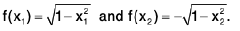
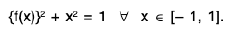
Example 3: Let f be a continuous function on [- 1, 1] such that (f(x)}2 + x2 + 1 for all x in [-1, 1]. Show th at either f(x) = √1- x2 for all x in [ - 1 , 1] or f(x) = -√1- x2 for all x in [ - 1 , 1 ].
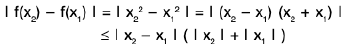
Sol: Let, if possible, there exists two points x,, x2 in [ - 1, 1] such that
Then f(x1) f(x2) < 0.
Since f is continuous in [- 1, 1] so f is continuous in [x1, x2] and f(x1) f(x2) < 0. By Theorem ∃ some c ∈ (x1, x2) such that f(c) = 0.
We are given
In particular, {(f(x)}2 + c2 = 1 (∴ c ∈ ( - 1, 1 ))
⇒ c2 = 1 (∴ f(c) = 0)
⇒ c = ± 1, which is impossible.
Example 4: Discuss the nature of discontinuity of the function f defined by 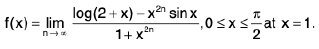 Show that f(0) and f(π/2) differ in sign and explain why f still does not vanish in
  .
.
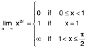
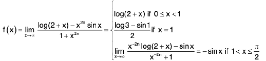
Sol: First of all we obtain expressions for f in
in a form free from limits.
Since∴
Now
Sincef(x) and
f(x) both exist, but are unequal, also neither of them is equal to f(1), therefore, f has a discontinuity of the first kind at x = 1 on both sides.
Now f(0) = log 2 > 0 and
So that f(0) and f(π/2) have opposite signs. Also, it is clear that f does not vanish anywhere in
The function f is not continuous on, the point x = 1 being a point of discontinuity. This explains the reason why f does not vanish anywhere
even though f(0) and f(π/2) are of opposite signs.


Remark. The above example shows that the hypothesis as well as the conclusion of the Intermediate value Theorem are not satisfied for the function f in 
Ex :Show that the function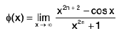 does not vanish anywhere in the interval [0, 2], though ϕ(0) and ϕ(2) differ in sign.
Hint.We have f(x) = - cos x for 0 ≤ x < 1 ;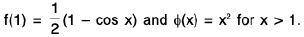
f(0) = -1 < 0, ϕ(2) = 4 > 0.
Verify that ϕis discontinuous at x = 1.
Example 5: Given an example of a function which satisfies the conclusion but not the hypothesis of the Intermediate value theorem.
Sol: We defined a function f on [0, 1] as follows :
Then f is not continuous in [0, 1] except at x =1/2
However, f takes every value between 0 and 1.
Uniform Continuity
A function f defined on an interval I is said to be uniformly continuous in the interval I, if for each ε > 0, there exists some δ > 0 such that
I f(x2) - f(x1) I < ε, when I x2 - x2 I < d and for all x1, x2 ε I.
Remarks.
- It may be noted that whereas continuity of a function is defined at a point, the uniform continuity of a function is defined in an interval. Even when we say that a function f is continuous in an interval it means that f is continuous at all points of the interval.
- In case of continuity of a function at a point c, the choice of δ > 0 depends upon ε > 0 and the point c. But in case of uniform continuity of a function in an interval, the choice of δ > 0 depends only on ε > 0 and not on a pair of points of the given interval.
- A function f is not uniformly continuous in an interval I, if there exists some ε > 0, such that for any δ > 0, there exists a pair of points x, y ε I for which I f(x) - f(y) | > c, when I x - y | < δ.
Solved Example
Example 1: The function defined by f(x) = x2 is uniformly continuous in (- 2, 2 ).
Sol: Let ε > 0 be any number and x1, x2 ε (- 2, 2 ). Then
∴
or
Hence the function f is uniformly continuous in (- 2, 2).


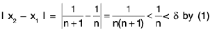
Example 2: Is the function f(x) =  uniformly continuous for x ∈ [0, 2] ? Justify your answer.
Sol: Let x, y be two arbitrary points x = [0, 2]. Then x ≥ 0, y ≥ 0
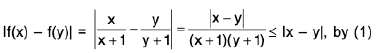
⇒ x + 1 ≥ 1 and y + 1 ≥ 1 ⇒ (x + 1)(y + 1) ≥ 1 ...(1)
Now
Let ε > 0 be given. Taking δ = ε, we see thatlf(x) - f(y)| < e, whenever lx - y| < δ, ∀ x, y ∈ [0, 2].
Hence f is uniformly continuous in [0, 2].
Example 3: Show that the function f defined by f(x) = x3 is uniformly continuous in the interval [0, 3].
Sol: Let ε > 0 and x1, x2 ∈ [0, 3] ∴x1 ≤ 3, x2 ≤ 3.
Now
=
=
∴
or I f(x2) - f(x1) I < ε, whenever I x2 — x1 I < ε/27.
Hence f is uniformly continuous in [0, 3].

Example 4: Show that f(x) = x2 is not uniformly continuous on [0, ∞)
Sol: Let ε = 1/2 and δ by any positive number. We can choose a positive integer n such that
...(1)
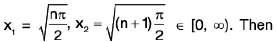
Let x, = √n and x2 = √n + 1 ∈ [0, ∞). Then
and
=
The I f(x2) - f(x1) I > ε, when I x2 - x1 I < δ.Hence f is not uniformly continuous on [0, ∞).

Example 5: Let f(x) = x2, x ∈ R. Show that f is uniformly continuous on every closed and finite interval but is not uniformly continuous on R.
Sol: Let [a, b] be any closed and finite interval. Let x1, x2 ∈ [a, b]. We have
Let k = max { I x1 I, I x2 I }. Then k > 0.
∴ I f(x2) - f(x1) I < 2k I x2 - x1 I.
Let ε > 0 be given and let δ = ε /2k > 0. Then
I f(x2) - f(x1) I < ε, whenever I x2 - x1 I < δ, ∀ x1x2 ∈ [a, b].
Hence f is uniformly continuous on [a, b].
However, f is not uniformly continuous on R.

Example 6: Show that f(x) = 1/x is not uniformly continuous on (0, 1].
Sol: Let ε = 1/2 and δ be any positive number. We can choose a positive integer n such that
---(1)
Letand
∈ (0, 1). Then
and
∴ I f(x2) - f(x1) I > ε, when I x2 - x1 I < δ.
Hence 1/x is not uniformly continuous on (0, 1].
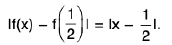
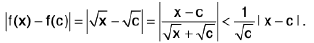
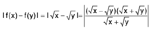
Example 7: Show that f(x) = √x is uniformly continuous in [0, 1].
Sol: Let x, y ∈ [0, 1], where x > y ≥ 0. Then
=
∴
Let ε > 0 be given. Then
I f(x) - f(y) I < ε, when √x-y < εor I f(x) - f(y) | < ε, when I x - y | < δ = (= ε2) ∀ x, y ∈ [0, 1].
Hence f is uniformly continuous in [0, 1].
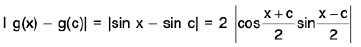
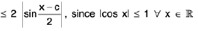
Example 8: Show that sin x is uniformly continuous on [0, ∞).
Sol: Let ε > 0 be given and x, y be any two points in [0, v). Let f(x) = sin x. Then
I f(x) - f(y) | = | sin x - sin y |
=
=
∴ I f(x) - f(y) | < I x - y |
⇒ I f(x) - f(y) | < ε, when I x - y | < δ, (δ = ε) ∀ x, y ∈ [0, ∞)
Hence f(x) = sin x is uniformly continuous on [0, ∞).

Example 9: Prove that f(x) = sin x2 is not uniformly continuous on [0, ∞)
Sol: Let ε= 1/2 and δ be any positive number. We can choose a positive integer n such that
...(1)
Let
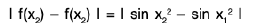
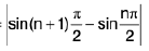
=
=
∴
and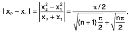
∴when I x2 - x, I < δ.
Hence f(x) = sin x2 is not uniformly continuous on [0, ∞).

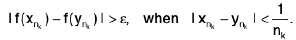
Example 10: Show that f(x) = sin1/x is not uniformly continuous on (0, ∞).
Sol: Let ε = 1/2 and δ be any positive number. We can choose a positive integer n such that
nπ / 1/8. ...(1)
Let
Then
Hence f(x) = sin1/x is not uniformly continuous on (0, ∞).

Theorem :Every uniformly continuous function on an interval is continuous on that interval, but the converse is not true.
Proof. Let a function f be uniformly continuous on an interval I. Then for any ε> 0, there exists some δ > 0 such that
Let c be any point of I. Taking y = c in (1), we obtainThus f is continuous at the point c.
Since c ∈ I is arbitrary, it follows that f is continuous at each point of I. Hence f is continuous on the interval I.
However, the converse of the theorem is not true.
A function which is continuous on an interval may not be uniformly continuous on that interval.
For example, the function f(x) = 1/x ∀ x ∈ (0, 1] is continuous on (0, 1], but f is not uniformly continuous on (0, 1].


However, if a function is continuous on a closed interval, then it is necessarily uniformly continuous on that closed interval as proved in the following :
Theorem : If a function f is continuous on a closed and bounded interval [a, b], then it is uniformly continuous on [a, b].
Proof. Let, if possible, f be not uniformly continuous on [a, b]. Then there exists some ε > 0 such that for any δn = 1/n (n ∈ N), there is a pair of elements xn, yn ∈[a, b] for which
Since a < xn ≤ b, a ≤ yn ≤ b for each n, the sequences <xn) and (yn) are bounded and so by Bolzano-Weierstrass theorem, they have limit points. Let a and p be limit points of <xn>, <yn) respectively. It follows that α and β are limit points of [a, b]. Since a closed interval is a closed set and further a closed set contains all its limit points, so α, β ∈ [a, b].
Now a is a limit point of <xn> implies that there exists a subsequence (xnk) of (xn) such that
xnk→a. ...(2)
Similarly, ynk → p, where (ynk) is a subsequence of <yn>. ...(3)
From (1), we conclude that
It is clear that
or lim xnk = lim ynk ⇒ α = β, by (2) and (3).
Butprovided the two limits exist.
It follows that f is not continuous at α ∈ [a, b], which is a contradiction to the given hypothesis. Hence f must be uniformly continuous in [a, b].

Solved Example
Example 1: If f and g are uniformly continuous on an interval I, then prove that f + g is uniformly continuous on I.
Sol: Since f and g are uniformly continuous on I, for any ε > 0, ∃ some δ1, > 0 and δ2 > 0 such that ∀ x, y ∈ I.
Let 8 = min (δ1, δ2). ...(3)
Now I (f + g) (x) - (f + g) (y) | = | (f(x) - f(y)} + (g(x) - g(y)} | ≤ I f(x) - f(y) | + | g(x) - g(y) |
∴∀x, y ∈ I ; using (1), (2) and (3).
Hence f + g is uniformly continuous in I.

Example 2: If f is uniformly continuous in an interval I and <xn> is a Cauchy sequence of elements in I, then <f(xn)> is a Cauchy sequence.
Sol: Since f is uniformly continuous in I, for any ε > 0,there exists some δ>0 such that ∀ x,y ∈ I,
Since <xn) is a Cauchy sequence in I, for ε = 8 > δ, ∃ a positive integer m such that
From (1) and (2), we obtain
Hence <f(xn)> is a Cauchy sequence.


Example 3: Prove that if f is uniformly continuous on a bounded interval I, then f is bounded on I.
Sol: Let, if possible, f be not bounded on I. Then for each n ∈ N, there exists some xn ∈ I such
that
---(1)
Since I is a bounded interval and xn ∈ I ∀ n ∈ N, <xn> is a bounded sequence in I. By Bolzano-Weierstrass Theorem, <xn) of <xn> has a limit point, say /. Then there exists a subsequence (xnk) of (xn) such that xnk → / as k → ∞ ⇒ (xn) is convergent and so (xn) is a Cauchy sequence in I. Since f is uniformly continuous on I, (f(xnk)) is a Cauchy sequence and hence f(xn)\ is bounded. From (1), we obtainfor all positive integers k
⇒ ( f (xnk) ) is not bounded, which is a contradiction.
Hence f is bounded on I.
Example 4: Justify with an example that the product of two uniformly continuous functions may not be uniformly continuous.
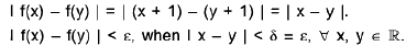
Sol: We shall prove that f(x) = x + 1 is uniformly continuous on R. Let ε > 0 be given. Then for any x, y ∈ R ; we have
Thus f(x) = x + 1 is uniformly continuous on R.
Similarly, g(x) = x - 1 is uniformly continuous on R.
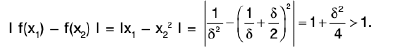
We shall now prove that f(x) g(x) = x2 - 1 is not uniformly continuous on R. For and δ > 0, letThen
and
If we choose c = 1, then I f(x1) - f(x2) I ≤ ε for I x1 - x2 I < δ. Hence the product x2 - 1 of two uniformly continuous functions x + 1 and x - 1 on R is not uniformly continuous on R.
Differentiability of a Function of One Variable
A function f is differentiable at an interior point x0 of its domain if the difference quotient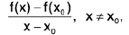
approaches a finite limit as x approaches x0, in which case the limit is called the derivative of f at x0 and is denoted by f’(xn); thus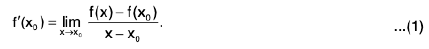 It is sometimes convenient to let x = x0 + h and write (1) as
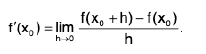 If f is defined on an open set S, we say that f is differentiable on S if f is differentiable at every point of S. If f is differentiable on S, then f’ is a function on S. We say that f is continuously differentiable on S if f is continuous on S. If f is differentiable on a neighborhood of x0, it is reasonable to ask if f is differentiable at x0. If so, we denote the derivative of f at x0 be f”(x0). This is the second derivative of f at x0, and it is also denoted by
  Continuing inductively, if f(n-1) is defined on a neighborhood of x0, then the nth derivative of f at x0, denoted by f<n> (x0) is the derivative of f(n-1) at x0. For convenience we defined the zeroth derivative of f to be f itself; thus
f<0> = f.
We assume that you are familiar with the other standard notations for derivatives; for example,
f(2) = f", f(3) = f" and so on, and 
Let f be a real valued function defined on an interval [a, b] i.e.,
f : [a, b] → R
Let a < c < b.
Definition : The left hand derivative of a function f at x = c, denoted by L f’(c) or f (c - 0) is defined as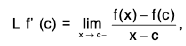 provided the limit exists.
Definition : If L f' (c) = R f' (c) then f is differentiable at x = c.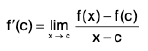
Definition :A function f defined on an interval [a, b] is said to be differentiable in the interval [a,b], if f is differentiable at all points of the interval [a, b].
Ex : If n is a positive integer and
f(x) = xn,
then
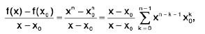
so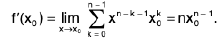
Since this holds for every x0, we drop the subscript and write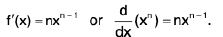
Interpretations of the Derivative
If f(x) is the position of a particle at time x ≠ x0 the difference quotient ...(1)
is the average velocity of the particle between times x0 and x. As x approaches x0, the average applies to shorter and shorter intervals. Therefore, it makes sense to regard the limit (1), if it exists, as the particle’s instantaneous velocity at time x0. This interpretation may be useful even if x is not time, so we often regard f’(x0) as the instantaneous rate of change of f(x) at xv regardless of the specific nature of the variable x. The derivative also has a geometric interpretation. The equation of the line through two points (x0, f(x0)) and (x1, f(x1)) on the curve y = f(x) (figure) is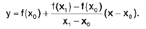 Varying x1 generates lines through (x0 f(x0)) that rotate into the line
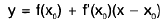
as x, approaches x0. This the tangent to the curve y = f(x) at the point (x0, f(x0)). Figure depicts the situation for various values of x1.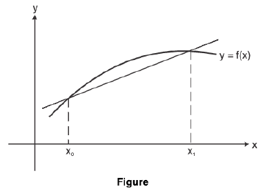
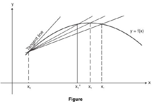 Here is a less intuitive definition of the tangent line: If the function
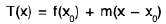 ...(1)
approximates f so well near x0 such that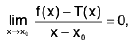
we say that the line y = T(x) is tangent to the curve y = f(x) at (x0, f(x0)).
This tangent line exists if and only if f’(x0) exists, in which case m is uniquely determined by m = f’(x0). Thus, (2) is the equation of the tangent line.
We will use the following lemma to study differentiable functions.
Lemma : If f is differentiable at x0, then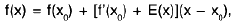
where E is defined on a neighborhood of x0 and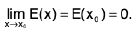
Theorem : Differentiability implies Continuity.
Proof. Let f be differentiable at x = c, so that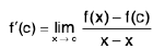
Now 
= 
= f’(c) x 0 = 0.
∴  Hence f is continuous at x = c.
The converse may not be true.
The function f(x) = I x I is continuous at x = 0 but not differentiable at x = 0.
We know 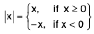
Now 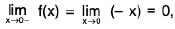
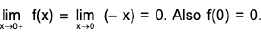
∴ 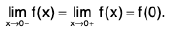
Hence f is continuous at x = 0.
Now 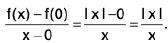
∴ 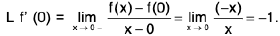
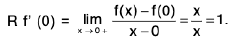
Thus L f’ (0) * R f (0) implies f is not differentiable at x = 0.
Solved Example
Example 1: Show that the function f(x) = x I x I is differentiable at the origin.
Sol: We have
∴ L f (0) = R f (0) = 0.
Hence f (0) = 0
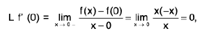
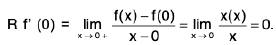
Example 2: Let f be defined by setting 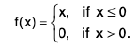 Show that f is differentiable at all points except x = 0.
Sol: We have
Since L f’(0) ≠ R f’(0), f is not differentiable at x = 0. Obviously f’(x) = 1, if x < 0 and f(x) = 0, if x > 0. Hence f is differentiable at all points except x = 0.
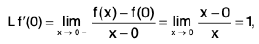
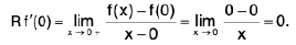
Example 3: Discuss the differentiability of the function 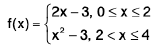 at x = 2, 4.
Sol: We have
Since L f' (2)≠ R f'(2), f is not differentiable at x = 2.
Since the given function is defined on [0, 4], therefore f (4) = L f' (4) = 8. Hence f is differentiable at x = 4.
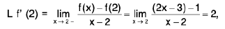
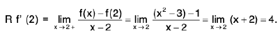

Example 4: Discuss the differentiability of the function 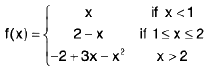 at x = 1, 2.
Sol:
∴
Hence f is not differentiable at x = 1.
Now
=
∴
Hence f is differentiable at x = 2 and f'(2) = -1.
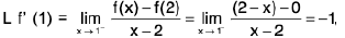
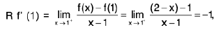
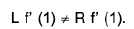
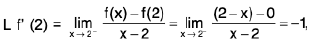
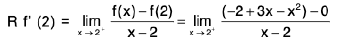
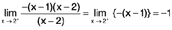
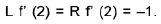
Example 5: Prove that the function defined as 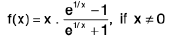 = 0, if x = 0 is not differentiable at x = 0. Further show that f is continuous at x = 0.
Sol: We have
(∴f(0) = 0)
=which doe s not exist.
Thus f is not differentiable at x = 0.
Now we show that f is continuous as x = 0.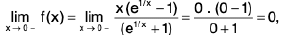
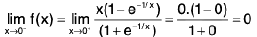
Also f(0) = 0. Hence f is continuous at x = 0.
Example 6: Examine the function f where 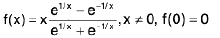 as regards continuity and differentiability at the origin.
Sol: We have
which does not exist.
Thus f is not differentiable at x = 0.
Now
=
Also f(0) = 0. Hence f is continuous at x = 0.
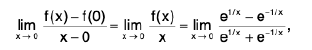
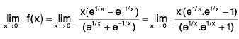

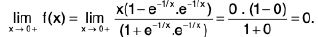
Example 7: If f(x) = x2 sin (1/x) when x ≠0 and f(0) = 0, show that f is differentiable for every value of x but the derivative is not continuous for x = 0.
Sol: We have
...(1)
So f’(0) = 0, which means f is differentiable at x = 0.
For x ≠ 0 , f'(x) = 2x sin (1 /x) + x2 cos (1/x) ( - 1/x2)
f'(x) = 2x sin (1/x) - cos (1/x). ...(2)
Hence f is differentiable for every value of x.
Now we discuss the continuity of f at x = 0. We have
Sincedoes not exist, it follows that f' is not continuous at x = 0.
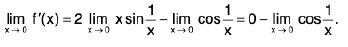
Example 8: If f(x) = 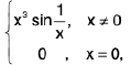 prove that f(x) has a derivative at x = 0 and that f(x) and f’(x) are continuous at x = 0.
Sol: We know
Also f(0) = 0.
∴ f’(0) = 0 and so f(x) is differentiable at x = 0. ...(1)
Now
=
Soimplies that f(x) is continuous at x = 0.
Now
=
∴
= = 0 x 0 - 0 = 0 = f' (0), by (1)
Soimplies that f (x) is continuous at x = 0.
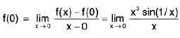
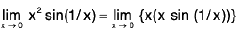

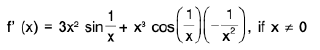
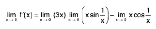
Example 9: Let f be defined on R by setting f(x) = x4sin (1/x), if x ≠ 0 and f(0) = 0. Show that f"(0) exists but f" is not continuous at x = 0.
Sol: We have
=
Thus f(0) = 0. Nowf’(x) = 4x3 sin (1/x) - x2 cos (1/x), x * 0.
f”(x) = [12 x2 sin (1/x) - 4x cos (1/x)] - [2x cos (1/x) + sin (1/x)]
or f”(x) = 12 x2 sin (1/x) - 6x cos (1/x) - sin (1/x).
Now
=which does not exist
Thus f” is not continuous at x = 0. Now
=
=
Hence f”(0) exists but f is not continuous at x = 0.
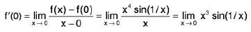


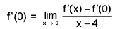
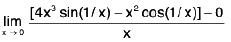
Example 10: Show that the function f defined by 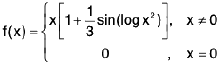 is continuous at x = 0 but not differentiable at x = 0.
Sol: We have
Let ε > 0 be given and δ = 3ε/4. Then
I f(x) - f(0) | < ε, if I x - 0 | < δ. Hence f is continuous at x = 0.
Now
=
=which does not exist.
Hence f is not differentiable at x = 0.
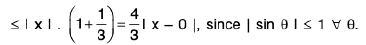
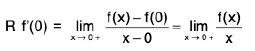
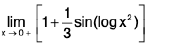
Example 11: Show that the function f defined as f(x) = I x - 1 | + |x+1 | ∀ x ∈ R is not differentiable at the points x = -1 and x = 1, and is differentiable at every other point.
Sol: We have I x - 1 | = x - 1, if x ≥ 1
and I x - 1 | = - (x - 1), if x < 1.
Also l x + 1 I = x + 1, if x ≥ - 1 and | x + 1 | = - (x + 1), if x < 1.
∴
Let
=
Since L f'(- 1) ≠ R f'(- 1), f is not differentiable at x = -1.
Now
Since L f'(1) ≠ R f'(1), f is not differentiable at x = 1.
From (1) f'(x) = - 2 ∀ x < - 1 .From (2), f'(x) = 0, if - 1 < x < 1.
From (3), f'(x) = 2 ∀ x > 1.
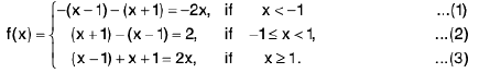
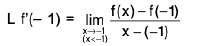
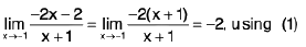
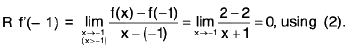
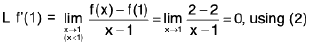
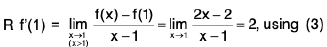
Algebra of Derivatives
Theorem: If f and g be two functions which are defined on [a, b] and differentiable at any point c ∈ [a, b], then
(f + g)’ (c) = f (c) + g’ (c).
Further for each real number k, the function kf is also differentiable at c and
(kf)’ (c) = kf' (c).
Proof. (i) Since f and g are differentiable at c, therefore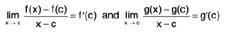 ...(1)
Consider 
= 
= 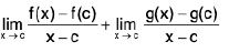
= f (c) + g’ (c), using (1).
Hence f + g is differentiable at c and (f + g)’ (c) = f (c) + g’ (c).
(ii)Now 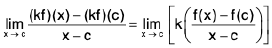
= 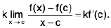
Hence kf is differentiable at c and (kf)’ (c) = kf'(c).
Theorem :If f and g are two differentiable functions at x = c, then fg also differentiable at x = c and (fg)’ (c) = f(c) g’(c) + g(c) f(c).
Proof. Since f and g are differentiable at x = c, therefore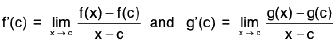 ...(1)
Since f and g are differentiable at x = c, so f and g are continuous and x = c. Thus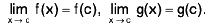 ...(2)
Now 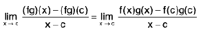
= 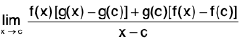
= 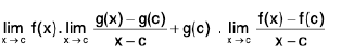
= f(c) g’(c) + g(c) f(c), using (1) and (2).
Hence fg is differentiable at c and
(fg)’ (c) = f(c) g’(c) + g(c) f’(c).
Theorem : (i) If a function f is differentiable at c and if f(c) ≠ 0, then 1/f is also differentiable at c and 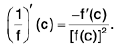
(ii) If f and g be two functions on [a, b] and differentiable at any point c ∈ [a, b] and if g(c) * 0, then f/g is also differentiable at c and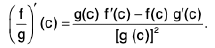
Proof, (i) Since f is differentiable at c, so f is continuous at c.
Thus 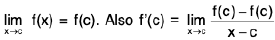
Now 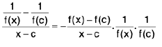
∴ 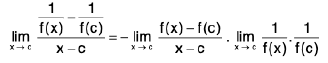
= 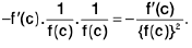
Hence 1/f is differentiable at c and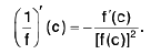 ...(2)
(ii) Since g is differentiable at c and g(c) ≠ 0. So 1/g is differentiable at c. By Theorem , we see that
f and 1/g and differentiable at c ⇒ f. 1/g is differentiable at c.
Hence f/g is differentiable at c. Again by Theorem, we have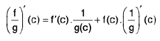
= 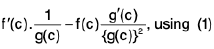
Hence, 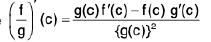
Theorem : (Chain Rule)
Let f: I → R and g : J → R be real-valued functions defined on the intervals I and J, respectively such that f(l) ⊂ J. Let f be differentiable at c ∈ I and g be differentiable at f(c). Then gof is differentiable at c and
(gof)’ (c) = g’ (f(c)).f'(c).
Theorem (Inverse Function Theorem for Derivatives)
Let f be a continuous one-to-one function defined on an interval and let f be differentiable at x0 with f'(x0)≠ 0. Then the inverse of the function f is differentiable at f(x0) and its derivative at f(x0) is 1/f’(x0).
The proof is omitted.
Solved Example
Example 1: Let f and g be two functions having the same domain D. If fg is differentiable at x0 ∈ D, is it necessary that f and g are both differentiable at xn? Give argument in support of your answer.
Sol: The function f and g may not be both differentiable at x0.
Let f(x) = I x I and g(x) = - | x | ∀ x ∈ 1 .Then (fg)(x) = f(x ) g(x) = - | x |2 = - x2. ( ∴ I x I2 = x2)
Obviously, fg is differentiable at x = 0, since
(fg )’(x) = - 2x and ( fg )’(0) = 0.
But f and g are both not differentiable at 0.
Example 2: Let f and g be two functions having the same domain D. If f ± g and f/g are differentiable at x0 ∈ D, is it necessary that f and g are both differentiable at x0?
Sol: (i) The functions f and g may not be both differentiable at x0.
Let
Let g(x) = - f ( x ) ∀ x ∈ R.Then (f + g) (x) = f(x) + g(x) = 0 ∀ x ∈ R.
∴ f + g is differentiable at 0 and (f + g)’ (0) = 0.
But f and g are both not differentiable at 0.
(ii)Let f(x) = g(x) = I x I ∀ x ∈ RThen (f - g) (x) = f(x) - g(x) = 0 ∀ x ∈ R.
Obviously, f - g is differentiable at x = 0 and (f - g)’ (0) = 0.
But f and g are both not differentiable at x = 0.
(iii) Let
Then f and g are both not differentiable at 0. But
is differentiable at x = 0.
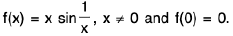

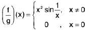
Example 3: Let f(x) = I x I and g(x) = 3 I x I. Show that f and g are not differentiable at the origin. But  exists and is equal to
Sol: We know that f and g are not differentiable at the origin (x = 0).
Now
We have f(x) = x, if x ≥ 0 and f(x) = - x, if x < 0,
and g(x) = 3x, if x ≥ 0 and g(x) = -3x, if x < 0.
Clearly,
Now
Hence
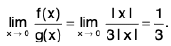
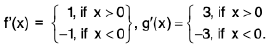
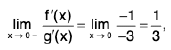
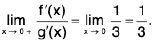
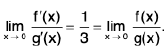
Example 4: Let f and g be two functions with domain D satisfying g(x) = x f(x) ∀ x ∈ D. Show that if f be continuous at x = 0 ∈ D, then g is differentiable at x = 0.
Sol: We have
since f is continuous at x = 0.
Hence g’(0) = f(0), which shows that g is differentiable at x = 0.
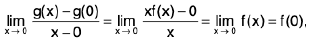
Sign of the Derivative
Suppose a function f is defined in [a, b] and f'(c) exists for any point c ∈ [a, b]. Let f'(c) > 0.
Since  = f’(c), so for ε > 0, ∃ some δ > 0, such that
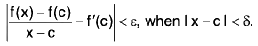
⇒ 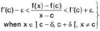 ...(1)
Let us choose ε > 0 so that ε < f’(c) ⇒ f(c) > ε ⇒ f(c) - ε > 0 ...(2)
From (1 ), we consider 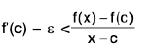
⇒ 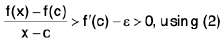
⇒ 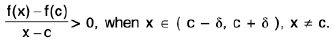
⇒ (x) - f(c) > 0, when x ∈ ( c , c + δ ) (∴ x > c)
and f(x) - f (c) < 0, when x ∈ ( c - δ, c ). (∴ x < c)
∴ 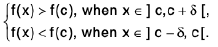
Hence 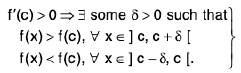 ...(A)
This property is often stated as follows :
If f’(c) > 0, then f is increasing at c.
Let f'(c) < 0.
We define a function g as follows :
g(x) = - f(x) ∀ x ∈ [a, b].
Then g ’(c) = - f (c) > 0.
Now g’ (c) > 0 ⇒ ∃ some δ > 0 such that ..(B)
g(x) > g(c) ⇒ f(x) < f(c) ∀x ∈ ( c, c + δ ),
g(x) < g(c) ⇒f(x) > f(c) ∀x ∈ ( c - δ, c ).
In other words,
If f'(c) < 0, then f is decreasing at c.
We now consider the end points. It may be show that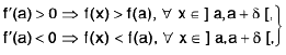 ...(C)
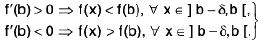 ...(D)
Note :The students are strongly advised to remember the results (A), (B), (C) and (D) as these will be frequently used.
Darboux’s Theorem
Theorem :If a function f defined in [a, b] is such that
(i) f is differentiable in [a, b]
(ii) f’ (a) and f (b) are of opposite signs, then there exists some point c e ( a, b ) such that f'(c) = 0.
Proof. Let us suppose that f'(a) > 0 and f'(b) < 0.
Since f’ (a) > 0 ⇒ ∃ some δ1 > 0 such that
f(x) > f(a), ∀ x ∈ ( a, a + 8, ). ...(1)
Since f'(b) < 0> ⇒ ∃ some δ2 > 0 such thatf(x) > f(b), ∀ x ∈ ( b - δ2, b ). ...(2)
Since f is differentiable in [a, b], f is continuous in [a, b] and hence bounded there in and the bounds are attained.
Let K = sup f and k = inf f. Then ∃ points c, d ∈ [a, b] such that
f(c) = K and f(d) = k. ...(3)
Now K = sup f ⇒ f(x) ≤ K, ∀ x ∈ [a, b]. ...(4)
We shall show that c ≠ a and c ≠ b.Let, if possible, c = a. Then f(c) = f(a) or K = f(a), using (3)
⇒
This contradicts (4). Thus c ≠ a.
Similarly, we can show that c ≠ b. Thus c ∈ (a, b ).
Finally, we show that f’(c) = 0.Case I.Let f' (c) > 0.
⇒∃ some δ3 > 0 such that f(x) > f(c), ∀ x ∈ ( c, c + δ3 )
⇒f(x) > K, ∀ x ∈ ( c, c + δ3 ), by (3)
This contradicts (4) and so f’(c) ≥ 0.
Case II. Let f' (c) < 0.⇒ ∃ some δ4 > 0 such that f(x) > f(c), ∀ x ∈ (c - δ3,c)
⇒ f(x) > K, ∀ x ∈ ( c - δ4, c ), by (3)
This contradicts (4) and so f’(c) < 0. Hence f’(c) = 0.

Remark.Darboux’s Theorem may be restated as follows :
Let f be defined and differentiable on [a, b]. If f'(a) f'(b) < 0, then there exists some point c ∈ ( a, b ) such that f' (c) = 0.
Proof. It is clear that
f’(a) f'(b) < 0 ⇒ f’(a) and f'(b) are of opposite signs.
Now proceed like Theorem.
Theorem.If f is differentiable in [a, b] and f’(a) ≠ f(b), then for each number k lying between f'(a) and f’(b), ∃ some point c ∈ ( a, b ) such that f' (c) = k.
Proof. We are given that f’ (a) < k < f' (b). ...(1)
Let g(x) = f(x) - kx ∀ x ∈ [a, b]. ...(2)
Since f is differentiable in [a,b] and kx is also differentiable in [a,b], therefore, by (2), g is differentiable in [a,b].
Now g'(x) = f'(x) - k ...(3)
⇒g’(a) = f'(a) - k < 0 and g'(b) = f'(b) - k > 0, by (1).
Thus g is differentiable in [a, b] and g’(a), g’(b) are of opposite signs. So by Darboux’s Theorem, ∃ some point c ∈ ( a, b ) such that
g’(c) = 0
⇒ f’(c) - k = 0, by (3)
Hence f’(c) = k.
Solved Example
Example 1: If f be differentiable at a point c, then show that I f I is also differentiable at c, provided f(c) ≠ 0. Show by means of an example that if f(c) = 0, then f may be differentiable at c and I f I may not be differentiable at c.
Sol: Since f is differentiable at c, f is continuous at c.
Now f(c) ≠ 0 ⇒ f(c) > 0 or f(c) < 0.
Consequently, ∃ δ1 > 0 and δ2 > 0 such that
or
Thusor
In either case, it follows that I f I is differentiable at c, since f is differentiable at c. However, I f I may not be differentiable at c, if (c) = 0.
For example let f(c) = x ∀ x ∈ R. Then f(0) = 0 and
I f(x) 1 = 1x1 ∀ x ∈ R.
Clearly, I f I is not differentiable at x = 0, although f is differentiable at x = 0.
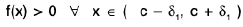
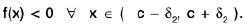
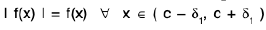

Example 2: If f be defined and differentiable on [a, b], f(a) = f(b) = 0, and f’(a) and f' (b) are of the same sign, then prove that f must vanish at least once in ( a, b ).
Sol: We are given that f(a) = f(b) = 0.
Since f'(a) and f'(b) are of the same sign, we may take
f’(a) > 0 and f'(b) > 0.
Now f’(a) > 0 ⇒ ∃ some δ1 > 0 such that
f(x) > f(a) = 0 ∀ x ∈ ( a, a + δ1 ].
Again f’(b) > 0 ⇒ ∃ some δ2 > 0 such that
f(x) > f(b) = 0 ∀ x ∈ [b - δ2, b).
Thus f(a + δ1) > 0 and f(b - δ2) < 0. ...(1)
Obviously, [a + δ1, b - δ2 ] ⊂ [a, b]. ...(2)
Since f is differentiable in [a, b], f is continuous in [a, b] and consequently by (2), f is continuous in [a + δ1, b - δ2], where f(a + δ1) and f(b - δ2) are of opposite signs, by (1). Hence by Theorem , there exists some c e ( a + δ1)( b - δ2) ⊂ ( a, b ) such that f(c) = 0. Hence f must vanish at least once in (a, b).
Example 3: If f is differentiable on [a, b], f(a) = f(b) = 0, and f(x) ≠ 0 for any x in(a, b), then prove that f’(a) and f’(b) must be of opposite signs.
Sol: Let, if possible, f’(a) and f'(b) be of the same sign. Also f(a) = f(b) = 0. By Example there exists some c ∈ (a, b) such that f(c) = 0. This contradicts the given hypothesis that f(x) ≠ 0 for all x in (a, b). Hence f’(a) and f'(b) must be of opposite signs.
Example 4: Let f : [- 1, 1] → R be defined by 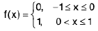 . Does there exists a function g such that g’(x) = f(x) ∀ x ∈ [- 1, 1] ?
Sol: Let, if possible, there exist a function g : [ - 1, 1] → R such that
It follows that g is differentiable on [ - 1, 1] and g ’ (-1) * g ’(1) [∴ g’(-1) = 0 and g’(1) = 1].
By Theorem g’ must assume every value between 0 and 1. [∴ g’(-1) = 0 and g’(1) = 1.]
But this is impossible, since
g ’(x) = 1 ∀ x ∈ (0, 1).
Hence there does not exist any function g such that
g’(x) = f(x) ∀ x ∈ [-1, 1].
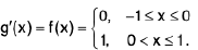
Intermediate Value Property
A real function is said to have the intermediate value property on an interval [a, b] if, for each value v between f(a) and f(b), there is some c ∈ (a, b) such that f(c) = v. Thus, a function with the intermediate value property takes all intermediate values between any two points.
The simplest, and most important, examples of functions with this property are the continuous functions.
Theorem by (Intermediate Value Theorem)
If a function f is continuous in [a, b] and f(a) ≠ f(b), then f assumes every value between f(a) and f(b).
Proof. Suppose that f(a) < f(b) and let M be any number lying between f(a) and f(b), i.e., f(a) < M < f(b) ...(1)
We have to show that ∃ some point c ∈ [a, b] such that f(c) = M.
Let us define a function ϕ on [a, b] as follows :
ϕ(x) = f(x) - M, ∀ x ∈ [a, b] ...(2)
Since f is given to be continuous in [a, b] and M being a constant is always continuous, so ϕ is continuous in [a, b].
From (2), ϕ(a) = f(a) - M and ϕ(b) = f(b) - M.
By (1), f(a) - M < 0 and f(b) - M > 0
⇒ ϕ(a) and ϕ(b) are of opposite signs,
By Theorem there exists some point c ∈ ( a, b ) such that
ϕ(c) = 0 ⇒ f(c) - M = 0, by (2)
Hence f(c) = M, c ∈ ( a, b ).
Remark. If a function f is not continuous on a closed interval, then the conclusion of the Intermediate Value Theorem may not hold:
Consider a function on [0, 1] as follows:
f(x) = x + 1 ∀ x ∈ ( 0, 1 ].
f(0) = 0.
Obviously, f is continuous on (0, 1]. Further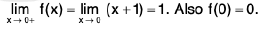
∴ 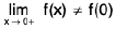 and so f is not continuous at 0.
i.e., f is not continuous in the closed interval [0, 1].
Now f(0) = 0, f(1) = 2.
We see that f(0) < 1 < f(1). But there does not exist y any x ∈ (0, 1] such that f(x) = 1.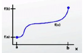
Ex. Is there a solution to x5 - 2x3 - 2 = 0, where x ∈ [0, 2] ?
At x = 0, we have 05 - 2 x 03 - 2 = -2.
At x = 2, we have 25 - 2 x 23 - 2 = 14.
So that IVT implies that there is a solution to x5 - 2x3 - 2 = 0 in the interval [0, 2].
Ex. Suppose that f is continuous on [0, 1] and f(0) = f(1). Let n be any positive integer, then prove that there is some number x such that
Define g(x) = 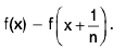
Consider the set of numbers S = 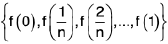
Let k be such that  is the largest number in S. Suppose that k ≠ 0 and k≠ n.
then 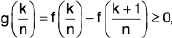 and
and 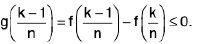
By the Intermediate value theorem, there is  with g(c) = 0, so that
 = 0 or
  as desired.
Finally, if the largest number in S is f(0) = f(1), then the same argument works with k chosen such that f (k/n) is the minimum number in S.
Note that if f(0) is both the largest and smallest number in S, then they are all the same and 
Suppose that f is continuous on [0, 1] and f(0) = f(1). Let c be the hyperreal unit, then prove that there is some number x such that f(x) = f(x + ε).
First, assume f(x) is not constant on [0, 1]. The result holds trivially if it is.
Then, let g(x) = f(x) - f(x + ε).
Since f is not constant, there exists a c ∈ [0, 1] such that f(c) is a maximum (or a minimum, but assume for now that it is a max, a min is handled similarly).
Then g(c) = f(c) - f(c + ε) > 0 and g(c - ε) = f(c -ε) - f(c) < 0
Now, by the Intermediate Value Theorem, if ε > 0, there exists a y <∈ [c - ε, c] such that
g(y) = 0.
(If ε < 0, y ∈ [c, c - ε], instead.)
Thus, f(y) = f(y + ε), as wanted.
If ε = 0, f(x) = f(x +ε) ∀x
Solved Example
Example 1: Apply intermediate value property to show that the equation x5 - 3x2 = -1 has a solution in the interval [0, 1].
Sol: Let f(x) = x5 - 3x2. Then f(x) is a continuous function with f(0) = 0 and f(1) = -2. As -1 is a value between -2 and 0, the intermediate value property of continuous functions indicates that f(x) = -1 must have a solution in the interval [0, 1].
Example 2: Apply intermediate value property to show that the equation x5 - 5x3 + 3 = 0 has a solution in the interval [-1, 1].
Sol: Let f(x) = x5 - 5x3 + 3. Then f(x) is a continuous function with f(-1) = 7 and f(1) = -1. As 0 is a value between -1 and 7, the intermediate value property of continuous functions indicates that f(x) = 0 must have a solution in the interval [-1, 1].
Example 3: Apply intermediate value property to show that the equation √x6 +5x4 +9 = 3.5 has a solution in the interval [0, 1].
Sol: Let f(x) = √x6 +5x4 +9 . Then f(x) is a continuous function with f(0) = 3 and f(1) = 4. As 3.5 is a value between 3 and 4, the intermediate value property of continuous functions indicates that f(x) = 3.5 must have a solution is the interval [0, 1].
Example 4: Show that the equation (1 - x)cosx = sinx has at least one solution in (0, 1).
Sol: Set f(x) = (1 - x)cosx - sinx. Then f(0) = 1 and f(1) = -sin1 < 0. By the intermediate value property there is x0 ∈ (0, 1) such that f(x0) = 0.
Example 5: Let f : [0, 1] → [0, 1] be continuous. Show that f has a fixed point in [0, 1]; that is, there exists x0 ∈ [0, 1] such that f(x0) = x0.
Sol: Define the function g(x) = f(x) - x on [0, 1]. Then f is continuous, g(0) ≥ 0 and g(1) ≤ 0. Use the intermediate value property (IVP).
Example 6: Let f : [a, b] → R be a continuous function. Show that the range {f(x) : ∈ [a, b]} is a closed and bounded interval.
Sol: Since f is a continuous function, there exist x0, y0 ∈ [a, b] such that f(x0) = m = inf f and f(y0) = M = sup f. Suppose x0 < y0. By the IVP, for every a e [m, M] there exists x ∈ [x0 y0] such that f(x) = a. Hence f[(a, b]) = [m, M].
Example 7: Show that a polynomial of odd degree has at least one real root.
Sol: Let p(x) = anxn + an-1xn-1 + ... + a1x + a0, an ≠ 0 and n be odd. Then p(x) =
+ +
If an >0, then p(x) → ∞ as x → oo and p(x) → -∞ as x→-∞. Thus by the IVP, there exists x0 such that p(x0) = 0. Similar argument for an < 0.
|
98 videos|34 docs|32 tests
|
FAQs on Functions of One Variable - I - Mathematics for Competitive Exams
| 1. What is a real-valued function and how is it defined? |  |
| 2. How do you perform arithmetic operations on functions? | |
| 3. What is the domain of definition of a function? | |
| 4. Can you explain what a bounded function is? | |
| 5. What are piecewise functions and how are they represented? | |


Objective type Questions
,Extra Questions
,Functions of One Variable - I | Mathematics for Competitive Exams
,practice quizzes
,study material
,video lectures
,MCQs
,Functions of One Variable - I | Mathematics for Competitive Exams
,Viva Questions
,mock tests for examination
,Important questions
,Semester Notes
,Free
,ppt
,Summary
,Functions of One Variable - I | Mathematics for Competitive Exams
,Exam
,shortcuts and tricks
,Sample Paper
,Previous Year Questions with Solutions
,past year papers
;


Functions of One Variable - I Free PDF Download
Importance of Functions of One Variable - I
Functions of One Variable - I Notes
Functions of One Variable - I Mathematics Questions
Study Functions of One Variable - I on the App
|
© EduRev
|
Education Revolution
|


|


