Basic Concepts of Root Locus


Introduction
The root locus method was introduced by W. R. Evans in 1948. It is a graphical technique used to determine how the closed-loop poles of a linear time-invariant feedback system move in the complex s-plane as a chosen parameter varies. The parameter most commonly varied is the loop gain of the system.
Consider a standard single-loop feedback arrangement with forward transfer function G(s) and feedback transfer function H(s).
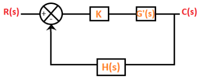
Characteristic Equation and the Role of Gain
The closed-loop characteristic equation of the system is
1 + G(s)H(s) = 0
If the forward path contains a variable scalar gain K, it is convenient to write G(s) = K G'(s). The characteristic equation then becomes
1 + K G'(s) H(s) = 0
When the parameter K varies, the roots of the characteristic equation (the closed-loop poles) move in the s-plane. Two common ranges for K are:
- -∞ to +∞ - the complete root locus (both negative and positive K values).
- 0 to +∞ - the direct root locus (most commonly used in engineering design).
The locus traced by all possible closed-loop pole locations as K varies over the chosen range is called the root locus. When K varies from zero to infinity, the plot is called the direct root locus. When K varies from -∞ to zero, the plot is the inverse root locus. Unless otherwise stated, K is usually taken from 0 to +∞.
Example
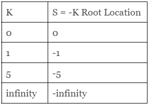
Example: Obtain the root locus of the unity feedback system with G(s) = K/s.
Solution
As the system is unity feedback, H(s) = 1.
Write the characteristic equation:
1 + G(s)H(s) = 0
Substitute G(s) = K/s and H(s) = 1:
1 + K/s = 0
Multiply by s to clear the denominator:
s + K = 0
The closed-loop pole satisfies:
s = -K
Since K varies from 0 to +∞ (direct root locus), the closed-loop pole moves along the negative real axis from the origin toward -∞ as K increases.
Basic Definitions and Relationships
- Open-loop poles and zeros: Poles and zeros of G(s)H(s) determine the starting and ending points of root locus branches. Each branch starts at an open-loop pole (K = 0) and ends at an open-loop zero (K → ∞). If there are fewer finite zeros than poles, the remaining branches tend to zeros at infinity.
- Number of branches: Equal to the number of open-loop poles (counting multiplicity).
- Branch start and end points: Start at open-loop poles for K = 0 and terminate at open-loop zeros for K → ∞ (finite zeros) or at infinity if no finite zero exists for that branch.
- Direct vs inverse root locus: Direct root locus shows movement for K from 0 to +∞; inverse root locus shows movement for K from -∞ to 0.
Rules for Sketching Root Locus (Standard Practical Rules)
1. Real-axis segments
On the real axis, a point is part of the root locus if the number of real open-loop poles and zeros to its right is odd. Mark the real-axis poles and zeros and identify the segments that satisfy this rule.
2. Number of branches
The number of branches of the root locus equals the number of open-loop poles (counting multiplicities). Each branch originates at a pole when K = 0.
3. Asymptotes (when number of poles n > number of zeros m)
If n - m = r branches go to infinity, they do so along straight line asymptotes. The angles of these asymptotes are
φq = (2q + 1) × 180° / (n - m) for q = 0, 1, 2, ..., (n - m - 1).
The centroid (intersection point) of the asymptotes on the real axis is
σ = (Σ poles - Σ zeros) / (n - m)
4. Angle condition
For a point s to lie on the root locus (for some K), the open-loop transfer function must satisfy the angle condition:
∠G'(s)H(s) = (2k + 1) × 180°, where k is any integer.
In practice, compute the angles contributed by each zero and each pole at the point s and verify the net angle equals an odd multiple of 180°.
5. Magnitude condition and determination of K
Once a point s0 satisfies the angle condition, the required gain K that places a closed-loop pole at s0 is found from the magnitude condition:
K = 1 / |G'(s0) H(s0)|
6. Breakaway and break-in points
Breakaway (or break-in) points occur on the real-axis segments where multiple branches meet or split. They satisfy the condition obtained by differentiating the characteristic equation with respect to s and solving for s when K is real and positive:
From 1 + K G'(s) H(s) = 0, express K = -1 / (G'(s)H(s)).
Find values of s on the real axis where dK/ds = 0. Real solutions that lie on the root locus are breakaway or break-in points.
7. Angles of departure/arrival for complex poles/zeros
For a complex pole p, the angle of departure θd is computed so that the net angle condition at p is satisfied. The angle of arrival to a complex zero z is computed similarly. These angles are obtained from the contributions of all other poles and zeros.
8. Imaginary-axis crossings
To find values of K at which the root locus crosses the imaginary axis, substitute s = jω into the characteristic equation and separate real and imaginary parts, then solve for ω and K. The Routh-Hurwitz criterion provides an alternative systematic method to find the range of K for stability and the exact crossing points.
9. Multiple and repeated roots
If the system has repeated poles or zeros, special care is required at those locations; repeated poles are locations where branches may depart with symmetric angles and multiplicity influences local behaviour.
How to Use the Angle and Magnitude Conditions (Worked Guidance)
To test whether a point s0 is on the root locus:
- Compute the sum of angles from s0 to each zero and subtract the sum of angles from s0 to each pole.
- Check that the resulting angle equals (2k + 1)180° for some integer k (angle condition).
- If the angle condition is satisfied, compute K from the magnitude condition K = 1 / |G'(s0)H(s0)|.
Applications of Root Locus
- Stability analysis: The root locus shows whether closed-loop poles move into the left half of the s-plane with increasing gain and thus whether the system is stable.
- Damping ratio and natural frequency: Positions of poles give the damping ratio (ζ) and natural frequency (ωn) of dominant modes, which determine transient response characteristics.
- Gain selection: Determine values of gain K that achieve desired pole locations, damping ratios or settling times.
- Controller design (P, PI, PID): Root locus is used to choose controller gains and to place additional poles/zeros so that closed-loop poles lie in acceptable regions.
- Compensator design (lead, lag): Adding zeros (lead compensator) or poles (lag compensator) modifies the root locus path so desired closed-loop behaviour can be obtained.
- Performance metrics: Root locus plots help estimate gain margin, phase margin, transient response and settling time trends as gain varies.
Advantages and Practical Remarks
- Root locus provides a visual and intuitive way to study how pole locations change with gain and how stability and transient response are affected.
- It permits straightforward determination of gain values that produce specified closed-loop pole locations using the magnitude condition.
- Asymptote and centroid formulae give useful asymptotic behaviour for high gain when zeros are fewer than poles.
- Root locus is useful even for systems with time delay or higher order dynamics; additional rules or numerical plotting tools are typically used in such cases.
- It complements frequency-domain methods (Bode, Nyquist) and state-space design techniques; choice depends on design requirements and ease of use.
Illustrative Design Remarks
When designing controllers using root locus:
- Place added zeros to pull the locus to the left (improve stability and speed) and place poles to shape low-frequency gain or steady-state behaviour.
- Use root locus to find the smallest gain that achieves a required damping ratio for dominant poles.
- Combine graphical root locus sketches with algebraic checks (Routh criterion, exact K from magnitude condition) for final verification.
Summary
The root locus is a foundational tool in classical control design. Using the characteristic equation 1 + K G'(s) H(s) = 0, the angle condition and magnitude condition determine whether a point in the s-plane belongs to the locus and the corresponding gain. Practical sketching rules (real-axis segments, asymptotes, breakaway points, departure/arrival angles) together with algebraic checks allow engineers to analyse stability and design controllers (P, PI, PID, lead/lag) to meet dynamic specifications.
FAQs on Basic Concepts of Root Locus
| 1. What is the characteristic equation in control systems? |  |
| 2. How does gain affect the root locus of a system? | |
| 3. What are the basic rules for sketching root locus? | |
| 4. What are the angle and magnitude conditions in root locus analysis? | |
| 5. What are the advantages of using root locus methods in control system design? | |


 | Explore Courses for Electrical Engineering (EE) exam |
 | Get EduRev Notes directly in your Google search |