Shortest Remaining Time First (SRTF) CPU Scheduling Algorithm

Table of Contents
1. Introduction
2. Key terms
3. How SRTF works (high level)
4. Pseudocode (simple view)
5. Properties, advantages and disadvantages
6. Example
7. When to use SRTF and implementation notes
8. Conclusion
View more

Introduction

The Shortest Remaining Time First (SRTF) scheduling algorithm is the preemptive form of Shortest Job First (SJF) scheduling. At any instant the short-term scheduler selects the ready process that has the smallest remaining CPU burst time. If a new process arrives whose remaining burst time is smaller than the remaining time of the currently running process, the running process is preempted; its context is saved in the Process Control Block (PCB) and the CPU is given to the newly arrived shorter job.

When all processes are already present in the ready queue (no further arrivals), SRTF behaves identically to non-preemptive SJF. Context switches occur when a running process is removed from the CPU; the process resumes later using the saved PCB information.

Key terms

• CPU burst time - total time a process requires on the CPU (also called service time).
• Arrival time - the time at which a process enters the ready queue.
• Remaining burst time - time still required by a process to complete.
• Preemption - interruption of a running process to schedule another.
• Ready queue - list of processes that are ready to execute but waiting for the CPU.
• Process Control Block (PCB) - data structure where the OS saves process state during preemption.
• Gantt chart - visual timeline showing which process runs on the CPU at each time interval.
• Waiting time - total time a process spends in the ready queue (not running).
• Turnaround time - total time from arrival to completion (finish time - arrival time).
• Response time - time from arrival to the first time the process gets the CPU.

How SRTF works (high level)

• When the CPU becomes free or when a new process arrives, the scheduler selects the process with the smallest remaining burst time from the ready queue.
• If the selected process differs from the currently running one, the current process is preempted and its PCB is updated.
• If multiple processes have equal remaining time, the tie is typically resolved by arrival time (earlier arrival chosen), or by an implementation-specific rule (e.g., FIFO among equals).
• When no new processes will arrive, SRTF reduces to SJF: the remaining process with the smallest remaining time runs to completion.
• SRTF tends to reduce average waiting time compared to non-preemptive policies, but it can cause starvation for long processes if short jobs keep arriving.

Pseudocode (simple view)

while there are unfinished processes: if ready queue is empty: advance time to next process arrival else: choose process p in ready queue with minimum remaining_time run p for one time unit (or until next arrival) decrement p.remaining_time if p.remaining_time == 0: mark p as finished and record finish time if a new process arrives with remaining_time < current remaining_time: preempt current process and put it back into ready queue

Properties, advantages and disadvantages

• Preemptive: immediate switching possible when a shorter job arrives.
• Low average waiting time: generally gives low average waiting time compared with many other policies for the same workload.
• Possible starvation: long processes may wait indefinitely if short jobs keep arriving.
• Context-switch overhead: frequent preemption increases context switching and associated overhead.
• Tie handling: requires a consistent tie-breaking rule (commonly arrival order).
• Implementation: needs up-to-date knowledge of remaining time; typically implemented with a priority queue keyed by remaining time.

Example

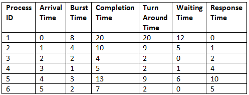
Consider six processes P1, P2, P3, P4, P5 and P6. Their arrival times and CPU burst times are given in the following table:

The Gantt chart for SRTF scheduling is constructed according to arrivals and remaining times. The scheduling events and decisions are described below.

• At time 0 only P1 has arrived with a CPU burst of 8 units. So P1 runs from time 0 to 1.
• At time 1 P2 arrives with burst 4. P1 has remaining 7 units; P2 (4) is smaller, so the CPU is given to P2.
• At time 2 P3 arrives with burst 2. P2 had remaining 3 at time 2; P3 (2) is smaller, so the CPU switches to P3.
• At time 3 P4 arrives. At this instant remaining times are: P1 = 7, P2 = 3, P3 = 1 (after one unit of P3), P4 = 1. Tied processes P3 and P4 both have remaining 1; P3 arrived earlier, so P3 is chosen and completes by time 4.
• At time 4 P5 arrives. P3 has finished; P4 has remaining 1 which is least, so P4 runs and finishes by time 5.
• At time 5 P6 arrives with burst 2. The remaining processes now are P1 (7), P2 (3), P5 (3), P6 (2). P6 (2) is the smallest; since all processes have arrived now, SRTF behaves like SJF for the remaining jobs. P6 runs to completion (t = 5-7), then P2 (3) runs (t = 7-10), then P5 (3) runs (t = 10-13), and finally P1 (7) runs (t = 13-20).

Gantt chart (timeline)

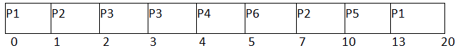
Using the decision sequence above the Gantt chart is:

0-1: P1    1-2: P2    2-4: P3    4-5: P4    5-7: P6    7-10: P2    10-13: P5    13-20: P1

Completion times, turnaround times and waiting times

Let us compute completion, turnaround and waiting times for each process. Use the relationships:

• Turnaround time = Finish time - Arrival time
• Waiting time = Turnaround time - CPU burst time

From the Gantt chart the finish times are: P1 = 20, P2 = 10, P3 = 4, P4 = 5, P5 = 13, P6 = 7.

The stepwise computation (each line is a logical step) is shown below.

Process P1:

Arrival time = 0

Burst time = 8

Finish time = 20

Turnaround time = 20 - 0 = 20

Waiting time = 20 - 8 = 12

Process P2:

Arrival time = 1

Burst time = 4

Finish time = 10

Turnaround time = 10 - 1 = 9

Waiting time = 9 - 4 = 5

Process P3:

Arrival time = 2

Burst time = 2

Finish time = 4

Turnaround time = 4 - 2 = 2

Waiting time = 2 - 2 = 0

Process P4:

Arrival time = 3

Burst time = 1

Finish time = 5

Turnaround time = 5 - 3 = 2

Waiting time = 2 - 1 = 1

Process P5:

Arrival time = 4

Burst time = 3

Finish time = 13

Turnaround time = 13 - 4 = 9

Waiting time = 9 - 3 = 6

Process P6:

Arrival time = 5

Burst time = 2

Finish time = 7

Turnaround time = 7 - 5 = 2

Waiting time = 2 - 2 = 0

Average waiting time

The sum of waiting times = 12 + 5 + 0 + 1 + 6 + 0 = 24

Number of processes = 6

Average waiting time = 24 ÷ 6 = 4 time units

When to use SRTF and implementation notes

• Use SRTF when the system goal is to minimise average waiting time and when preemption and precise remaining-time information are available and affordable.
• Because SRTF may perform many context switches, account for context-switch overhead when evaluating performance; very short jobs with heavy context switching may reduce overall throughput.
• To implement SRTF efficiently, maintain a min-heap or balanced tree keyed by remaining time so the shortest remaining job can be located quickly on each arrival.
• Provide starvation prevention if required (for example, by ageing or by switching to a multi-level feedback queue) when long processes must be guaranteed progress.

Conclusion

SRTF is a useful preemptive scheduling policy that minimises average waiting time in many workloads by always running the process with the least remaining CPU requirement. It needs careful handling of context-switch overhead and starvation. For the worked example above the algorithm produces an average waiting time of 4 time units, computed from a total waiting time of 24 across six processes.