Key Notes: Measures of Central Tendency | Economics Class 11 - Commerce PDF Download

Introduction
- The chapter discusses measures of central tendency, a numerical method to summarize data.
- Common examples include average marks, average rainfall, average production, and average income.
- Central tendency helps evaluate and compare data efficiently, such as the economic condition of farmers in a village.
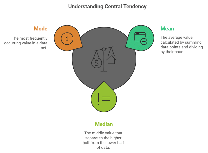
- Three primary measures of central tendency are:
- Arithmetic Mean
- Median
- Mode
- Other types include the Geometric Mean and Harmonic Mean, but the focus is on the three main averages.
Arithmetic Mean
The Arithmetic Mean is calculated by adding all values and dividing by the number of observations. For example, for monthly incomes of six families: 1600, 1500, 1400, 1525, 1625, 1630, the mean is:
- Sum = 1600 + 1500 + 1400 + 1525 + 1625 + 1630 = 8,280
- Mean = 8,280 / 6 = Rs 1,380
The formula for the Arithmetic Mean:
X = (X1 + X2 + X3 + ... + XN) / N
Where N = total number of observations.
Calculating the Arithmetic Mean
Ungrouped Data
- Direct Method: Simply sum all observations and divide by the total count. Example: Marks: 40, 50, 55, 78, 58 results in:
Mean = (40 + 50 + 55 + 78 + 58) / 5 = 56.2 - Assumed Mean Method: Useful for large datasets. Assume a mean (A), calculate deviations (d), and find the actual mean using:
X = A + (Σd / N)
Grouped Data
- Discrete Series: Multiply frequency by observation values, sum them up, and divide by total frequency:
Formula: X = Σ(fX) / Σf - Continuous Series: Use mid-points of class intervals for calculations, following a similar process as discrete data.
Properties of the Arithmetic Mean
- The sum of deviations from the mean is always zero: Σ(X - X) = 0.
- The mean is sensitive to extreme values, which can significantly affect its value.
Merits of the Arithmetic Mean
- Easy to compute: The arithmetic mean is calculated using basic mathematical operations such as addition, multiplication, and division, making it straightforward to determine.
- Simple to understand: The arithmetic mean is easy to grasp, as it effectively represents the average value per unit or cost per unit of a data set.
- Based on all items: It considers all values in the data set, providing a complete and comprehensive representation of the distribution of values.
- Rigidly defined: The arithmetic mean has a clear and definite value because it is calculated based on a fixed formula.
- A good basis for comparison: It serves as a reliable benchmark for comparing different groups of data, allowing for effective analysis of differences and similarities.
- Algebraic treatment: The arithmetic mean can be manipulated algebraically, making it a useful tool in more advanced statistical analyses.
Demerits of Arithmetic Mean
- Complete data is required: To calculate the arithmetic mean, all items in the data series must be available; missing data can lead to inaccuracies.
- Affected by extreme values: The arithmetic mean can be significantly influenced by outliers or extreme values, which can distort the average.
- Absurd results: In some cases, the arithmetic mean may yield illogical results, such as reporting a fractional number of students in a class, which is not meaningful.
- Calculation by observation is not possible: Unlike the median or mode, the arithmetic mean cannot be easily identified through mere observation of the data set.
- No graphic representation: The arithmetic mean does not lend itself to visual representation on graphs, making it less intuitive in some contexts.
- Not applicable for open-ended frequency distributions: It is not feasible to compute the arithmetic mean for open-ended frequency distributions without making assumptions about class sizes.
- Not applicable to qualitative characteristics: The arithmetic mean cannot be calculated for qualitative data, such as attributes related to intelligence, honesty, or habits, as these do not have numerical values.
Weighted Arithmetic Mean
- When different items have different importance, weights can be assigned to calculate a weighted mean.
- Formula:
Weighted Mean = (W1 * P1 + W2 * P2) / (W1 + W2)
Median
The median is the positional value that divides a data distribution into two equal parts.
It separates values into:
- Values that are greater than or equal to the median
- Values that are less than or equal to the median
- The median is the middle value when the dataset is sorted.
- It is not influenced by extreme values (outliers).
Computation of Median:
- Sort the data from smallest to largest.
- Find the middle value.
Example 1: For the data sets 5, 7, 6, 1, 8, 10, 12, 4, and 3:
- Sorted order: 1, 3, 4, 5, 6, 7, 8, 10, 12
- The median (middle score) is 6.
If the number of values is even, the median is the arithmetic mean of the two middle values.
Example 2: For marks of 20 students:
- Data: 25, 72, 28, 65, 29, 60, 30, 54, 32, 53, 33, 52, 35, 51, 42, 48, 45, 47, 46, 33
- Sorted order: 25, 28, 29, 30, 32, 33, 33, 35, 42, 45, 46, 47, 48, 51, 52, 53, 54, 60, 65, 72
- Two middle values: 45 and 46
- Median = (45 + 46) / 2 = 45.5 marks
To find the position of the median in an ordered data set, use the following formula:
- Position of median = (N + 1) / 2
- Where N = number of items.
Discrete Series: For discrete data, locate the median using cumulative frequency.
Example: Income data:
- Income (in Rs): 10, 20, 30, 40
- Number of persons: 2, 4, 10, 4
- Cumulative frequency table:
10: 2
20: 6
30: 16
40: 20 - Median position: (20 + 1) / 2 = 10.5
- The median income is Rs 30 (found in the cumulative frequency).
Continuous Series: Locate the median class where the N/2th item lies.
Use the formula:
- Median = L + [(N/2 - cf) / f] * h
- Where:
L = lower limit of the median class
cf = cumulative frequency of the class before the median class
f = frequency of the median class
h = class interval size
Example: Daily wages of factory workers:
- Daily wages (in Rs): 55-60, 50-55, 45-50, 40-45, 35-40, 30-35, 25-30, 20-25
- Number of workers: 7, 13, 15, 20, 30, 33, 28, 14
- Cumulative frequency table:
20-25: 14
25-30: 28
30-35: 33
35-40: 30
40-45: 20
45-50: 15
50-55: 13
55-60: 7 - The median class is 35-40 (80th item).
- Median daily wage = Rs 35.83.
Quartiles
Divide the data into four equal parts.
- Q1 (first quartile): 25% of items below it
- Q2 (second quartile/median): 50% of items below it
- Q3 (third quartile): 75% of items below it

Percentiles
Divide data into hundred equal parts.
- P50 is the median value.
- Example: Securing the 82nd percentile means you scored better than 82% of candidates.
Calculation of Quartiles: Similar method as for median.
- Q1 = (N + 1) / 4th item
- Q3 = 3(N + 1) / 4th item
Example 5: Marks of ten students:
- Marks: 22, 26, 14, 30, 18, 11, 35, 41, 12, 32
- Sorted: 11, 12, 14, 18, 22, 26, 30, 32, 35, 41
- Q1 = (10 + 1) / 4 = 2.75th item = 2nd item + 0.75 * (3rd item - 2nd item) = 12 + 0.75 * (14 - 12) = 13.5 marks.
Mode
The mode is a statistical measure that represents the most frequently occurring value in a data set. It is particularly useful when you want to identify the typical value around which the maximum concentration of items occurs.
- The term "mode" derives from the French word la Mode, meaning the most fashionable or popular value in a distribution.
- The mode is denoted by Mo and is defined as the value that appears most often in the data.
Computation of Mode:
- For a discrete series, the mode is the number that appears most frequently. For example, in the data set 1, 2, 3, 4, 4, 5, the mode is 4 because it appears twice, more than any other number.
- In a frequency distribution, for instance:
Variable: 10, 20, 30, 40, 50
Frequency: 2, 8, 20, 10, 5
The mode is 30 since it has the highest frequency of 20. - Data can have:
- Unimodal: One mode (e.g., the example above).
- Bimodal: Two modes (e.g., 1, 1, 2, 2, 3, 3, 4, 4 has no mode).
- Multimodal: More than two modes.
- No mode: If all values occur with equal frequency.
Continuous Series:
- In continuous frequency distributions, the modal class is the class with the highest frequency.
- The mode can be calculated using the following formula:
Mo = L + (D1 / (D1 + D2)) * h
Where:
L = lower limit of the modal class
D1 = frequency of the modal class - frequency of the class before it
D2 = frequency of the modal class - frequency of the class after it
h = width of the class interval - For example, to calculate the modal income from a cumulative frequency table:
- Convert the cumulative frequency to an exclusive frequency distribution.
- Identify the modal class (where the frequency is highest).
- Using the formula, calculate the mode.
Relative Position of Averages
The relationship between the three measures of central tendency is as follows:
If Me is the arithmetic mean, Mi is the median, and Mo is the mode, then:
- Me > Mi > Mo or Me < Mi < Mo depending on the distribution shape.
- The median is always positioned between the arithmetic mean and the mode.
Conclusion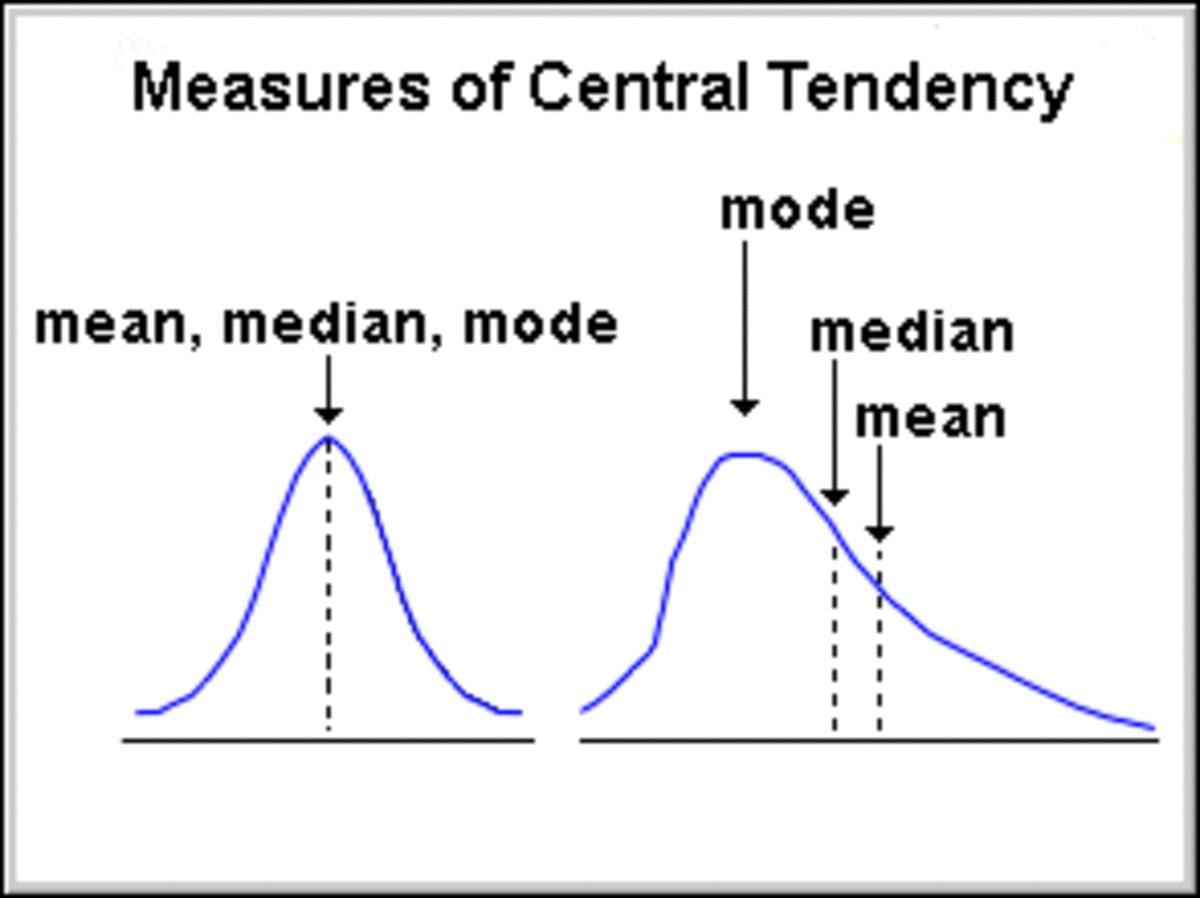
- Measures of central tendency provide a single value to summarise data.
- The arithmetic mean is the average most people use. It’s easy to calculate and considers all data points, but it can be skewed by very high or low values.
- The total of how much each item differs from the arithmetic mean always equals zero.
- A median is better when there are outliers, making it a more reliable summary for such data.
- For open-ended distributions, both the median and mode can be calculated easily.
- The mode is typically used for qualitative data description.
- Choosing the right average depends on what you are analysing and how the data is distributed.
|
59 videos|222 docs|43 tests
|
FAQs on Key Notes: Measures of Central Tendency - Economics Class 11 - Commerce
| 1. What are the three main measures of central tendency? |  |
| 2. How do you calculate the mean of a data set? | |
| 3. When is it more appropriate to use the median instead of the mean? | |
| 4. Can a data set have more than one mode? | |
| 5. How do you interpret the mode in a data set? | |


Extra Questions
,ppt
,MCQs
,practice quizzes
,Sample Paper
,Exam
,shortcuts and tricks
,Objective type Questions
,Free
,Key Notes: Measures of Central Tendency | Economics Class 11 - Commerce
,Semester Notes
,past year papers
,study material
,Previous Year Questions with Solutions
,Important questions
,video lectures
,Key Notes: Measures of Central Tendency | Economics Class 11 - Commerce
,mock tests for examination
,Viva Questions
,Key Notes: Measures of Central Tendency | Economics Class 11 - Commerce
,Summary
;


Key Notes: Measures of Central Tendency Free PDF Download
Importance of Key Notes: Measures of Central Tendency
Key Notes: Measures of Central Tendency
Key Notes: Measures of Central Tendency Commerce Questions
Study Key Notes: Measures of Central Tendency on the App
|
© EduRev
|
Education Revolution
|


|


