ICAI Notes- Unit 1: Law of Demand and Elasticity of Demand - 2 | Business Economics for CA Foundation PDF Download

Expansion and Contraction of Demand

The demand schedule, demand curve and the law of demand all show that when the price of a commodity falls, its quantity demanded increases, other things being equal. When, as a result of decrease in price, the quantity demanded increases, in Economics, we say that there is an expansion of demand and when, as a result of increase in price, the quantity demanded decreases, we say that there is a contraction of demand. For example, suppose the price of apples is ₹ 100/ per kilogram and a consumer buys one kilogram at that price. Now, if other things such as income, prices of other goods and tastes of the consumers remain the same but the price of apples falls to ₹ 80 per kilogram and the consumer now buys two kilograms of apples, we say that there is a change in quantity demanded or there is an expansion of demand. On the contrary, if the price of apples rises to ₹ 150 per kilogram and the consumer then buys only half a kilogram, we say that there is a contraction of demand. The phenomena of expansion and contraction of demand are shown in Figure 3. The figure shows that when price is OP, the quantity demanded is OM, given other things equal. When as a result of increase in price (O PII), the quantity demanded falls to OL, we say that there is ‘a fall in quantity demanded’ or ‘contraction of demand’ or ‘an upward movement along the same demand curve’. Similarly, as a result of fall in price to OPI , the quantity demanded rises to ON, we say that there is an ‘expansion of demand’ or ‘a rise in quantity demanded’ or ‘a downward movement on the same demand curve.’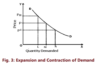

Increase and Decrease in Demand

Till now we have assumed that the other determinants of demand remain constant when we are analysing the demand for a commodity. It should be noted that expansion and contraction of demand take place as a result of changes in the price while all other determinants of price viz. income, tastes, propensity to consume and price of related goods remain constant. The ‘other factors remaining constant’ means that the position of the demand curve remains the same and the consumer moves downwards or upwards on it. There are factors other than price (non-price factors) or conditions of demand which might cause either an increase or decrease in the quantity of a particular good or service that buyers are prepared to demand at a given price. What happens if there is a change in consumers’ tastes and preferences, income, the prices of the related goods or other factors on which demand depends? As an example, let us consider what happens to the demand for commodity X if the consumer’s income increases: Table 3 shows the possible effect of an increase in income of the consumer on the quantity demanded of commodity X.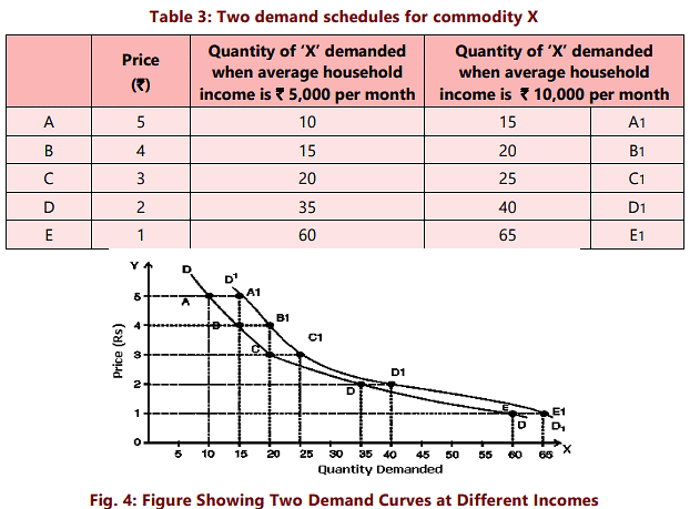

The two sets of data are plotted in Figure 4 as DD pertaining to demand when average household income is ₹ 5000/ and D’D’ when income is ₹ 10, 000/. We find that with increase in income, the demand curve for X has shifted [in this case it has shifted to the right]. The shift from DD to D’D’ indicates an increase in the desire to purchase ‘X’ at each possible price. For example, at the price of ₹ 4 per unit, 15 units are demanded when average household income is ₹ 5,000 per month. When the average household income rises to ₹ 10,000 per month, 20 units of X are demanded at price ₹ 4. You can find similar increase in demand at each price. Since this increase would occur regardless of what the market price is, the result would be a shift to the right of the entire demand curve. Alternatively, we can ask what price consumers would be willing to pay to purchase a given quantity, say 15 units of X. With greater income, they should be willing to pay a higher price of ₹ 5 instead of 4. A rise in income thus shifts the demand curve to the right, whereas a fall in income will have the opposite effect of shifting the demand curve to the left. Any change that increases the quantity demanded at every price shifts the demand curve to the right and is called an increase in demand. Any change that decreases the quantity demanded at every price shifts the demand curve to the left, and is called a decrease in demand. Figure 5(a) and (b) illustrate increase and decrease in demand respectively. When there is an increase in demand, the demand curve shifts to the right and more quantity will be purchased at a given price (Q1 instead of Q at price P). A decrease in demand causes the entire demand curve to shift to the left and we find that less quantity is bought at the same price P.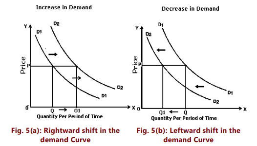

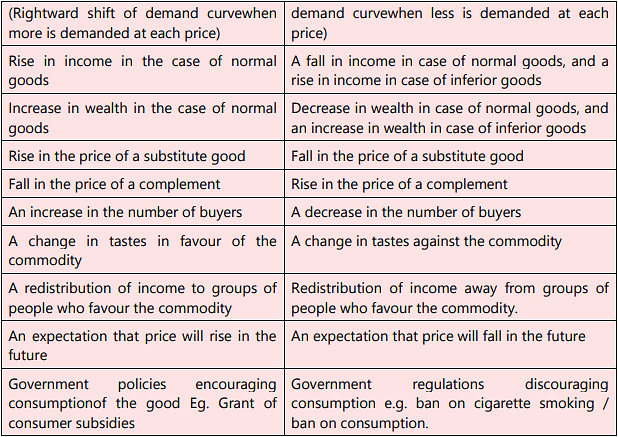
The table below summarises the effect of non - price determinants on demand

Movements along the Demand Curve vs. Shift of Demand Curve

It is important for the business decision-makers to understand the distinction between a movement along a demand curve and a shift of the whole demand curve.
A movement along the demand curve indicates changes in the quantity demanded because of price changes, other factors remaining constant. A shift of the demand curve indicates that there is a change in demand at each possible price because one or more other factors, such as incomes, tastes or the price of some other goods, have changed.
Thus, when an economist speaks of an increase or a decrease in demand, he refers to a shift of the whole curve because one or more of the factors which were assumed to remain constant earlier have changed. When the economists speak of change in quantity demanded he means movement along the same curve (i.e., expansion or contraction of demand) which has happened due to fall or rise in price of the commodity.
In short ‘change in demand’ represents shift of the demand curve to right or left resulting from changes in factors such as income, tastes, prices of other goods etc. and ‘change in quantity demanded’ represents movement upwards or downwards on the same demand curve resulting from a change in the price of the commodity. When demand increases due to factors other than price, firms can sell more at the existing prices resulting in increased revenue. The objective of advertisements and all other sales promotion activities by any firm is to shift the demand curve to the right and to reduce the elasticity of demand. (The latter will be discussed in the next section). However, the additional demand is not free of cost as firms have to incur expenditure on advertisement and sales promotion devices.

Elasticity of Demand

Till now we were concerned with the direction of the changes in prices and quantities demanded. From the point of view of a business firm, it is more important to know the extent of the relationship or the degree of responsiveness of demand to changes in its determinants. Often, we would want to know how sensitive is the demand for a product to its price; for example, if price increases by 5 percent, how much will the quantities demanded change? Also, how much change in demand will be there if the average income rises by 5 percent? What effect will an advertising campaign have on sales? Economists use a number of different types of elasticity to answer questions like these so as to make demand predictions and to recommend changes in strategies.

Consider the following situations:

1. As a result of a fall in the price of headphones from ₹ 500 to ₹ 400, the quantity demanded increases from 100headphones to 150 headphones. 
2. As a result of fall in the price of wheat from ₹ 20 per kilogram to ₹ 18 per kilogram, the quantity demanded increases from 500 kilograms to 520 kilograms. 
3. As a result of fall in the price of salt from ₹ 9 per kilogram to ₹ 7.50, the quantity demanded increases from 1000 kilogram to 1005 kilograms.

What do you notice? You notice that the demand for headphones, wheat and salt responds in the same direction to price changes. The difference lies in the degree of response of demand. The differences in responsiveness of demand can be found out by comparing the percentage changes in prices and quantities demanded. Here lies the concept of elasticity.
The amount of a commodity purchased is a function of many variables such as price of the commodity, prices of the related commodities, income of the consumers and other factors on which demand depends. A change in one of these independent variables will cause a change in the dependent variable, namely, the amount purchased per unit of time. The elasticity of demand measures the relative responsiveness of the amount purchased per unit of time to a change in any one of these independent variables while keeping others constant. In general, the coefficient of elasticity is defined as the proportionate change in the dependent variable divided by the proportionate change in the independent variable. Elasticity of demand is defined as the degree of responsiveness of the quantity demanded of a good to changes in one of the variables on which demand depends. More precisely, elasticity of demand is the percentage change in quantity demanded divided by the percentage change in one of the variables on which demand depends.
We may find different measures of elasticity such as price elasticity, cross elasticity, income elasticity, advertisement elasticity and elasticity of substitution. It is to be noted that when we talk of elasticity of demand, unless and until otherwise mentioned, we talk of price elasticity of demand. In other words, it is price elasticity of demand which is usually referred to as elasticity of demand.

Price Elasticity of Demand

Perhaps, the most important measure of elasticity of demand is the price elasticity of demand which measures the sensitivity of quantity demanded to ‘own price’ or the price of the good itself. The concept of price elasticity of demand is important for a firm for two reasons. 

• Knowledge of the nature and degree of price elasticity allows firms to predict the impact of price changes on its sales. 
• Price elasticity guides the firm’s profit-maximizing pricing decisions. 

Price elasticity of demand expresses the degree of responsiveness of quantity demanded of a good to a change in its price, given the consumer’s income, his tastes and prices of all other goods. In other words, it is measured as the percentage change in quantity demanded divided by the percentage change in price, other things remaining equal. The price elasticity of demand (also referred to as PED) tells us the percentage change in quantity demanded for each one percent (1%) change in price. That is,

The percentage change in a variable is just the absolute change in the variable divided by the original level of the variable.
Therefore,


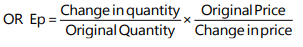
In symbolic terms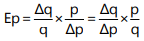

Where Ep stands for price elasticity q stands for original quantity p stands for original price ∆ stands for a change. A negative sign on the elasticity of demand illustrates the law of demand: less quantity is demanded as the price rises. Notice that the change in quantity was due solely to the price change. The other factors that potentially could affect sales (income and the competitor’s price) did not change. The greater the value of elasticity, the more sensitive quantity demanded is to price. Strictly speaking, the value of price elasticity varies from minus infinity to approach zero. This is because Δq/Δp has a negative sign. In other words, since price and quantity are inversely related (with a few exceptions) price elasticity is negative. While interpreting the coefficient of price elasticity, we consider only the magnitude of the price elasticity- i.e. its absolute size. For example, if Ep = -1.22, we say that the elasticity is 1.22 in magnitude. That is, we ignore the negative sign and consider only the numerical value of the elasticity. Thus if a 1% change in price leads to 2% change in quantity demanded of good A and 4% change in quantity demanded of good B, then we get elasticity of A and B as 2 and 4 respectively, showing that demand for B is more elastic or responsive to price changes than that of A. Had we considered minus signs, we would have concluded that the demand for A is more elastic than that for B, which is not correct. Hence, by convention, we take the absolute value of price elasticity and draw conclusions.

A numerical example for price elasticity of demand:

Illustration 1: The price of a commodity decreases from ₹ 6 to ₹ 4 and quantity demanded of the good increases from 10 units to 15 units. Find the coefficient of price elasticity.
Sol: Price elasticity = (-) Δ q / Δ p × p/q = 5/2 × 6/10 = (-) 1.5 

Illustration 2: A 5% fall in the price of a good leads to a 15% rise in its demand. Determine the elasticity and comment on its value.
Sol:

= 15% / 5% = 3

Illustration 3: The price of a good decreases from ₹ 100 to ₹ 60 per unit. If the price elasticity of demand for it is 1.5 and the original quantity demanded is 30 units, calculate the new quantity demanded.
Sol:

Here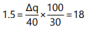

Therefore new quantity demanded = 30+18 = 48 units

Illustration 4: The quantity demanded by a consumer at price ₹ 9 per unit is 800 units. Its price falls by 25% and quantity demanded rises by 160 units. Calculate its price elasticity of demand.
Sol: Change in quantity demanded = 160
Therefore, % change in quantity demanded = 20%
% change in price = 25%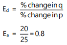

Illustration 5: A consumer buys 80 units of a good at a price of ₹ 4 per unit. Suppose price elasticity of demand is - 4. At what price will he buy 60 units?
So:

or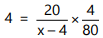

or

x = 4.2 per unit

Point Elasticity

The point elasticity of demand is the price elasticity of demand at a particular point on the demand curve. The concept of point elasticity is used for measuring price elasticity where the change in price is infinitesimal. Price elasticity is a key element in applying marginal analysis to determine optimal prices. Since marginal analysis works by evaluating “small” changes taken with respect to an initial decision, it is useful to measure elasticity with respect to an infinitesimally small change in price. Point elasticity makes use of derivative rather than finite changes in price and quantity. It may be defined as:

Where dq/dp is the derivative of quantity with respect to price at a point on the demand curve and p and q are the price and quantity at that point. Economists generally use the word “elasticity” to refer to point elasticity.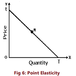

Point elasticity is, therefore, the product of price quantity ratio at a particular point on the demand curve and the reciprocal of the slope of the demand line.

Measurement of Elasticity on a Linear Demand Curve – Geometric Method

By definition, the price elasticity of demand is the change in quantity associated with a change in price (∆Q/∆P) times the ratio of price to quantity (P/Q) Therefore, the price elasticity of demand depends not only on the slope of the demand curve but also on the price and quantity. The elasticity, therefore, varies along the curve as price and quantity change. The slope of a linear demand curve is constant. However, the elasticity at different points on a linear demand curve would be different. When price is high price is high and quantity is small, the elasticity is high. The elasticity becomes smaller as we move down the curve.
Given a straight line demand curve tT, (Fig.6 above) point elasticity at any point say R can be found by using the formula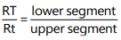

Using the above formula we can get elasticity at various points on the demand curve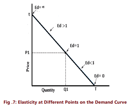

Thus, we see that as we move from T towards t, elasticity goes on increasing. At the midpoint it is equal to one, at point t, it is infinity and at T it is zero. 

Arc-Elasticity 

Often we may be required to calculate price elasticity over some portion of the demand curve rather than at a single point. In other words, the elasticity may be calculated over a range of prices. When price and quantity changes are discrete and large we have to measure elasticity over an arc of the demand curve.
When price elasticity is to be found between two prices (or two points on the demand curve say, A and B in figure 8) the question arises as to which price and quantity should be taken as base. This is because elasticity found by using original price and quantity figures as base will be different from the one derived by using new price and quantity figures. Therefore, in order to avoid confusion, rather than choose the initial or the final price and quantity, the mid-point method is used i.e. the averages of the two prices and quantities are taken as (i.e. original and new) base. The midpoint formula is an approximation to the actual percentage change in a variable, but it has the advantage of consistent elasticity values when price moves in either directions.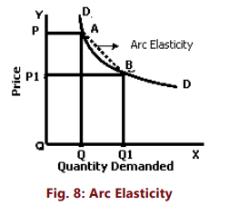

The arc elasticity can be found out by using the formula: We drop the minus sign and use the absolute value.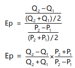

Where P₁, Q₁ are the original price and quantity and P₂, Q₂ are the new ones. Thus, if we have to find elasticity of demand for headphones between:
P₁ = ₹ 500 Q₁= 100
P₂ = ₹ 400 Q₂ = 150
We will use the formula
Or

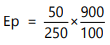
or
Ep =1.8
The arc elasticity will always lie somewhere (but not necessarily in the middle) between the point elasticities calculated at the lower and the higher prices.

Interpretation of the Numerical Values of Elasticity of Demand

Economists have found it useful to divide the demand behaviour into different categories, based on values of price elasticity. Since we draw demand curves with price on the vertical axis and quantity on the horizontal axis, ∆Q/∆P = (1/slope of curve). As a result, for any price and quantity combination, the steeper the slope of the curve, the less elastic is demand.
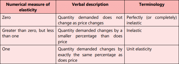
The numerical value of elasticity of demand can assume any value between zero and infinity. 

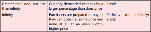
Elasticity is zero, (Ep= 0) if there is no change at all in the quantity demanded when price changes i.e. when the quantity demanded does not respond at all to a price change. In other words, any change in price leaves the quantity demanded unchanged and consumers will buy a fixed quantity of a good regardless of its price. Perfectly inelastic demand is as an extreme case of price insensitivity and is therefore only a theoretical category with less practical significance. The vertical demand curve in figure 8(a) represents perfectly or completely inelastic demand, Elasticity is one, or unitary, (Ep= 1) if the percentage change in quantity demanded is equal to the percentage change in price. Figure 8 (b) shows special case of unit-elastic demand, where the demand curve is a rectangular hyperbola. Elasticity is greater than one (Ep > 1) when the percentage change in quantity demanded is greater than the percentage change in price. In such a case, demand is said to be elastic. [Figure8 (d)]. In other words, the quantity demanded is relatively sensitive to price changes. When drawn, the elastic demand line is fairly flat. Elasticity is less than one (Ep < 1) when the percentage change in quantity demanded is less than the percentage change in price. In such a case, demand is said to be inelastic.[Figure 8 (e)]In this situation, when price falls the buyers are unable or unwilling to significantly contract demand. In other words, the quantity demanded is relatively insensitive to price changes. When drawn, the inelastic demand line is fairly steep. 

Elasticity is infinite, (Ep= ∞) when a ‘small price reduction raises the demand from zero to infinity. The demand curve is horizontal at the price level (where the demand curve touches the vertical axis). As long as the price stays at one particular level any quantity might be demanded. Moving back and forth along this line, we find that there is a change in the quantity demanded but no change in the price. If there is a slight increase in price, they would not buy anything from the particular seller. That is, even the smallest price rise would cause quantity demanded to fall to zero. Roughly speaking, when you divide a number by zero, you get infinity, denoted by the symbol∞. So a horizontal demand curve implies an infinite price elasticity of demand. This type of demand curve is found in a perfectly competitive market. The horizontal demand curve in figure 8 (c) represents perfectly or infinitely elastic demand,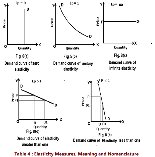

Now that we are able to classify goods according to their price elasticity, let us see whether the goods mentioned below are price elastic or inelastic.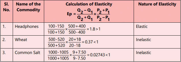

What do we note in the above hypothetical example? We note that the demand for headphones is quite elastic, while demand for wheat is quite inelastic and the demand for salt is almost the same even after a reduction in price.
The price elasticity of demand for the vast majority of goods is somewhere between the two extreme cases of zero and infinity. Generally, in real world situations also, we find that the demand for goods like refrigerators, TVs, laptops, fans, etc. is elastic; the demand for goods like wheat and rice is inelastic; and the demand for salt is highly inelastic or perfectly inelastic. Why do we find such a difference in the behaviour of consumers in respect of different commodities? We shall explain later at length those factors which are responsible for the differences in elasticity of demand for various goods. Before that, we will consider another method of calculating price-elasticity which is called total outlay method. 

Total Outlay Method of Calculating Price Elasticity 

The price elasticity of demand for a commodity and the total expenditure or outlay made on it are significantly related to each other. As the total expenditure (price of the commodity multiplied by the quantity of that commodity purchased) made on a commodity is the total revenue received by the seller (price of the commodity multiplied by quantity of that commodity sold of that commodity), we can say that the price elasticity and total revenue received are closely related to each other. By analysing the changes in total expenditure (or total revenue) in response to a change in the price of the commodity, we can know the price elasticity of demand for it. 

Price Elasticity of demand equals one or Unity: When, as a result of the change in price of a good, the total expenditure on the good or the total revenue received from that good remains the same, the price elasticity for the good is equal to unity. This is because the total expenditure made on the good can remain the same only if the proportional change in quantity demanded is equal to the proportional change in price. Thus, if there is a given percentage increase (or decrease) in the price of a good and if the price elasticity is unitary, total expenditure of the buyer on the good or the total revenue received from it will remain unchanged. 

Price elasticity of demand is greater than unity: When, as a result of increase in the price of a good, the total expenditure made on the good or the total revenue received from that good falls or when as a result of decrease in price, the total expenditure made on the good or total revenue received from that good increases, we say that price elasticity of demand is greater than unity. In our example of headphones, as a result of fall in price of headphones from ₹ 500 to ₹ 400, the total revenue received from headphones increases from ₹ 50,000 (500x100) to ₹ 60,000 (400 x 150), indicating elastic demand for headphones. Similarly, had the price of headphones increased from ₹ 400 to ₹ 500, the demand would have fallen from 150 to 100 indicating a fall in the total revenue received from ₹ 60,000 to ₹ 50,000 showing elastic demand for headphones. 

Price elasticity of demand is less than unity: When, as a result of increase in the price of a good, the total expenditure made on the good or the total revenue received from that good increases or when as a result of decrease in its price, the total expenditure made on the good or the total revenue received from that good falls, we say that the price elasticity of demand is less than unity. In the example of wheat above, as a result of fall in the price of wheat from ₹ 20 per kg. to ₹ 18 per kg. the total revenue received from wheat falls from ₹ 10,000 (20 x 500) to ₹ 9360 (18 x 520) indicating inelastic demand for wheat. Similarly, we can show that as a result of increase in the price of wheat from ₹ 18 to ₹ 20 per kg, the total revenue received from wheat increase from ₹ 9360 to ₹ 10,000 indicating inelastic demand for wheat. The main drawback of this method is that by using this we can only say whether the demand for a good is elastic or inelastic; we cannot find out the exact coefficient of price elasticity.
Why should a business firm be concerned about elasticity of demand? The reason is that the degree of elasticity of demand predicts how changes in the price of a good will affect the total revenue earned by the producers from the sale of that good. The total revenue is defined as the total value of sales of a good or service. It is equal to the price multiplied by the quantity sold. 

Total Revenue 

Total revenue (TR) = Price × Quantity sold 

Except in the rare case of a good with perfectly elastic or perfectly inelastic demand, when a seller raises the price of a good, there are two effects which act in opposite directions on revenue. 

• Price effect: After a price increase (decrease), each unit sold sells at a higher (lower) price, which tends to raise (lower) the revenue. 
• Quantity effect: After a price increase (decrease), fewer (more) units are sold, which tends to lower (increase) the revenue. 

What will be the net effect on total revenue? It depends on which effect is stronger. If the price effect which tends to raise total revenue is the stronger of the two effects, then total revenue goes up. If the quantity effect, which tends to reduce total revenue, is the stronger, then total revenue goes down.
The price elasticity of demand tells us what happens to the total revenue when price changes: its size determines which effect, the price effect or the quantity effect, is stronger.
If demand for a good is unit-elastic (the price elasticity of demand is equal to one; Figure 9), an increase in price or decrease in price does not change total revenue. In this case, the quantity effect and the price effect exactly balance each other. When price rises from P to P1, the gain in revenue (Area A) is equal to loss in revenue due to lost sales (Area B)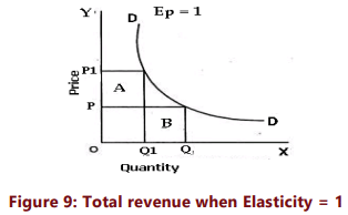

If demand for a good is inelastic (the price elasticity of demand is less than one), a higher price increases total revenue. In this case, the quantity effect is weaker than the price effect.
On the contrary, when demand is inelastic, a fall in price reduces total revenue because the quantity effect is dominated by the price effect. Refer Figure 8 (e) above.
If demand for a good is elastic (the price elasticity of demand is greater than one), an increase in price reduces total revenue and a fall in price increases total revenue. In this case, the quantity effect is stronger than the price effect. Refer Figure 8 (d) above.
Table 5 below summarizes the relationship between price elasticity and total revenue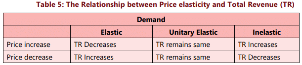

Determinants of Price Elasticity of Demand 

In the above section we have explained what price elasticity is and how it is measured. Now an important question is: What are the factors which determine whether the demand for a good is elastic or inelastic? We will consider the following important determinants of price elasticity. 

1. Availability of substitutes: One of the most important determinants of elasticity is the degree of substitutability and the extent of availability of substitutes. Some commodities like butter, cabbage, car, soft drink etc. have close substitutes. These are margarine, other green vegetables, other brands of cars, other brands of cold drinks respectively. A change in the price of these commodities, the prices of the substitutes remaining constant, can be expected to cause quite substantial substitution – a fall in price leading consumers to buy more of the commodity in question and a rise in price leading consumers to buy more of the substitutes. Commodities such as salt, housing, and all vegetables taken together, have few, if any, satisfactory substitutes and a rise in their prices may cause a smaller fall in their quantity demanded. Thus, we can say that goods which typically have close or perfect substitutes have highly elastic demand curves. Moreover, wider the range of substitutes available, the greater will be the elasticity. For example, toilet soaps, toothpastes etc have wide variety of brands and each brand is a close substitute for the other. It should be noted that while as a group, a good or service may have inelastic demand, but when we consider its various brands, we say that a particular brand has elastic demand. Thus, while the demand for a generic good like petrol is inelastic, the demand for Indian Oil’s petrol is elastic. Similarly, while there are no general substitutes for health care, there are substitutes for one doctor or hospital. Likewise, the demand for common salt and sugar is inelastic because good substitutes are not available for these. 
2. Position of a commodity in the consumer’s budget: The greater the proportion of income spent on a commodity; generally the greater will be its elasticity of demand and vice- versa. The demand for goods like common salt, matches, buttons, etc. tend to be highly inelastic because a household spends only a fraction of their income on each of them. On the other hand, demand for goods like rental apartments and clothing tends to be elastic since households generally spend a good part of their income on them. When the good absorbs a significant share of consumers’ income, it is worth their time and effort to find a way to reduce their demand when the price goes up. 
3. Nature of the need that a commodity satisfies: In general, luxury goods are price elastic because one can easily live without a luxury. In contrast, necessities are price inelastic. Thus, while the demand for a home theatre is relatively elastic, the demand for food and housing, in general, is inelastic. If it is possible to postpone the consumption of a particular good, such good will have elastic demand. Consumption of necessary goods cannot be postponed and therefore, their demand is inelastic. 
4. Number of uses to which a commodity can be put: The more the possible uses of a commodity, the greater will be its price elasticity and vice versa. When the price of a commodity which has multiple uses decreases, people tend to extend their consumption to its other uses. To illustrate, milk has several uses. If its price falls, it can be used for a variety of purposes like preparation of curd, cream, ghee and sweets. But, if its price increases, its use will be restricted only to essential purposes like feeding the children and sick persons. 
5. Time period: The longer the time-period one has, the more completely one can adjust. Time gives buyers the opportunity to find alternatives or substitutes, or change their habits. A simple example of the effect can be seen in motoring habits. In response to a higher petrol price, one can, in the short run, make fewer trips by car. In the longer run, not only can one make fewer trips, but he can purchase a car with a smaller engine capacity when the time comes for replacing the existing one. Hence one’s demand for petrol falls by more when one has made long term adjustments to higher prices.
6. Consumer habits: If a person is a habitual consumer of a commodity, no matter how much its price change, the demand for the commodity will be inelastic. If buyers have rigid preferences demand will be less price elastic. 
7. Tied demand: The demand for those goods which are tied to others is normally inelastic as against those whose demand is of autonomous nature. For example printers and ink cartridges. 
8. Price range: Goods which are in very high price range or in very low price range have inelastic demand, but those in the middle range have elastic demand. 
9. Minor complementary items: The demand for cheap, complementary items to be used together with a costlier product will tend to have an inelastic demand. Knowledge of the price elasticity of demand and the factors that may change it is of key importance to business managers because it helps them recognise the effect of a price change on their total sales and revenues. Firms aim to maximise their profits and their pricing strategy is highly decisive in attaining their goals. Knowledge of the price elasticity of demand for the goods they sell helps them in arriving at an optimal pricing strategy.
   If the demand for a firm’s product is relatively elastic, the managers need to recognize that lowering the price would expand the volume of sales and result in an increase in total revenue. On the contrary, when the demand is elastic, they have to be very cautious about increasing prices because a price increase will lead to a decline in total revenue as fall in sales would be more than proportionate. If the firm finds that the demand for their product is relatively inelastic, the firm may safely increase the price and thereby increase its total revenue as they can be assured of the fact that the fall in sales on account of a price rise would be less than proportionate.
   Knowledge of price elasticity of demand is important for governments while determining the prices of goods and services provided by them, such as, transport and telecommunication. Further, it also helps the governments to understand the nature of responsiveness of demand to increase in prices on account of additional taxes and the implications of such responses on the tax revenues. Elasticity of demand explains why the governments are inclined to raise the indirect taxes on those goods that have a relatively inelastic demand, such as alcohol and tobacco products.

Income Elasticity of Demand

The income elasticity of demand is a measure of how much the demand for a good is affected by changes in consumers’ incomes. Estimates of income elasticity of demand are useful for businesses to predict the possible growth in sales as the average incomes of consumers grow over time. Income elasticity of demand is the degree of responsiveness of the quantity demanded of a good to changes in the income of consumers. In symbolic form,

This can be given mathematically as follows: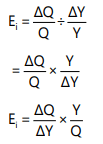

E_i = Income elasticity of demand
∆Q = Change in demand
Q = Original demand
Y = Original money income
∆Y = Change in money income
There is a useful relationship between income elasticity for a good and the proportion of income spent on it. The relationship between the two is described in the following three propositions: 

1. If the proportion of income spent on a good remains the same as income increases, then income elasticity for that good is equal to one. 
2. If the proportion of income spent on a good increase as income increases, then the income elasticity for that good is greater than one. The demand for such goods increase faster than the rate of increase in income.
3. If the proportion of income spent on a good decrease as income rises, then income elasticity for the good is positive but less than one. The demand for income-inelastic goods rises, but substantially slowly compared to the rate of increase in income. Necessities such as food and medicines tend to be income- inelastic 

The above stated propositions can be better understood with the help of the below example: Let, the price of a commodity is ₹ 10 per unit. Initially the consumer’s income is ₹ 100 and he spends @10% of his income i.e. ₹ 10 on the commodity demanding 1 unit of the same. Now, as the consumer’s income doubled to ₹200 (or increased by 100%), there may be three possibilities causing different degrees of income elasticity of demand as follows: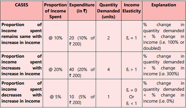

Income elasticity of goods reveals a few very important features of demand for the goods in question.
If income elasticity is zero, it signifies that the demand for the good is quite unresponsive to changes in income. When income elasticity is greater than zero or positive, then an increase in income leads to an increase in the demand for the good. This happens in the case of most of the goods and such goods are called normal goods. For all normal goods, income elasticity is positive. However, the degree of elasticity varies according to the nature of commodities.
When the income elasticity of demand is negative, the good is an inferior good. In this case, the quantity demanded at any given price decreases as income increases. The reason is that when income increases, consumers choose to consume superior substitutes. Another significant value of income elasticity is that of unity. When income elasticity of demand is equal to one, the proportion of income spent on goods remains the same as consumer’s income increases. This represents a useful dividing line. If the income elasticity for a good is greater than one, it shows that the good bulks larger in consumer’s expenditure as he becomes richer. Such goods are called luxury goods. On the other hand, if the income elasticity is less than one, it shows that the good is either relatively less important in the consumer’s eye or, it is a good which is a necessity.
The following examples will make the above concepts clear:
(a) The income of a household rises by 10%, the demand for wheat rises by 5%.
(b) The income of a household rises by 10%, the demand for T.V. rises by 20%.
 (c) The incomes of a household rises by 5%, the demand for bajra falls by 2%.
(d) The income of a household rises by 7%, the demand for commodity X rises by 7%.
(e) The income of a household rises by 5%, the demand for buttons does not change at all. 

Using formula for income elasticity

We will find income-elasticity for various goods. The results are as follows: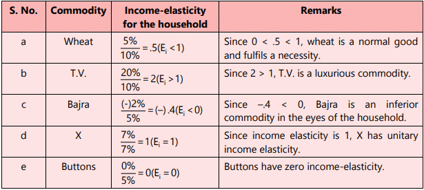
It is to be noted that the words ‘luxury’, ‘necessity’, ‘inferior good’ do not signify the strict dictionary meanings here. In economic theory, we distinguish them in the manner shown above. An important feature of income elasticity is that income elasticity differs in the short run and long run. For nearly all goods and services the income elasticity of demand is larger in the long run than in the short run Knowledge of income elasticity of demand is very useful for a business firm in estimating the future demand for its products. Knowledge of income elasticity of demand helps firms measure the sensitivity of sales for a given product to incomes in the economy and to predict the outcome of a business cycle on its market demand. For instance, if EY = 1, sales move exactly in step with changes in income. If EY >1, sales are highly cyclical, that is, sales are sensitive to changes in income. For an inferior good, sales are countercyclical, that is, sales move in the opposite direction of income and EY < 0. This knowledge enables the firm to carry out appropriate production planning and management.

Illustration 6

Income Elasticity of Demand
A car dealer sells new as well as used cars. Sales during the previous year were as follows: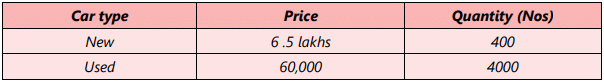
During the previous year, other things remaining the same, the real incomes of the customers rose on average by 10%. During the last year sales of new cars increased to 500, but sales of used cars declined to 3,850.
What is the income elasticity of demand for the new as well as used cars? What inference do you draw from these measures of income elasticity?
Sol:
Income Elasticity of demand for new cars
Percentage change in income = 10%, given
Percentage change in quantity of new cars demanded = (∆ Q/Q) X 100 = (100/400) X100 = 25%
Income elasticity of demand = 25%/ 10% = + 2.5
New car is therefore income elastic. Since income elasticity is positive, new car is a normal good.

Income Elasticity of demand for used cars 
Percentage change in income = 10%, given
% change in quantity of used cars demanded = (∆ Q/Q) X 100 = (-1 50/4000) x100 = - 3.75%- Income elasticity of demand = – 3.75/10= –.375
Since income elasticity is negative, used car is an inferior good.