Unit 2: Theory of Consumer Behaviour Chapter Notes | Business Economics for CA Foundation PDF Download
| Table of contents |

|
| Nature of Human Wants |

|
| Classification of Want |

|
| Relationship Between TU & MU |

|
| Law of Diminishing Marginal Utility |

|
| Consumer Surplus |

|
| Indifference Curve Analysis |

|
| Summary |

|
Nature of Human Wants
In economics, the term 'want' signifies a wish, desire, or motive to possess and utilize goods and services that provide satisfaction. Wants may arise from physical, psychological, or social influences. Due to limited resources, choices must be made between urgent and less urgent wants.All human wants exhibit certain characteristic features:
- Wants are unlimited in number; not all can be satisfied.
- Wants vary in intensity; some are urgent, while others are felt less intensely.
- “Utility” is influenced by the intensity of wants. Generally, utility refers to satisfaction, but in economics, it denotes the want-satisfying power of a commodity.
- Each want is satiable.
- Wants compete with one another for satisfaction due to the scarcity of resources.
- Wants can be complementary; some can only be fulfilled by using multiple goods or groups of goods.
- A specific want may be satisfied in various ways.
- Wants are subjective and relative, thus utility is also a subjective or relative concept.
- Wants change with time, place, and individual, affecting utility as well.
- Some wants recur, while others do not.
- Wants may evolve into habits and customs.
- Wants are influenced by income, tastes, fashions, advertisements, and social norms.
- Wants arise from diverse causes such as physical and psychological instincts, social obligations, and an individual's economic and social position.
Utility is a psychological notion, distinct from usefulness, and is not tied to moral or ethical values. Two important concepts of utility are Total Utility (TU) and Marginal Utility (MU), which are essential in consumer behavior theories:
- TU refers to the total utility gained from consuming all units of a commodity at a specific time, calculated as the sum of marginal utilities for all units consumed. Formula: TU = ∑ MU
- MU is the extra utility gained from consuming one more unit of a commodity. Formula: MU = TUn – TUn-1 or MU = ∆TU / ∆N
Classification of Want
In Economics, wants are classified into three categories: necessaries, comforts, and luxuries.Necessaries
Necessaries are essential for living and can be further divided into:
- Necessaries for life: Items required to meet the basic physiological needs for survival, such as minimum food, clothing, and shelter.
- Necessaries for efficiency: These go beyond mere survival and include nourishing food, proper clothing, clean water, comfortable housing, education, and recreation, which are necessary for maintaining longevity, energy, and work efficiency.
- Conventional necessaries: These arise from habitual pressures or social customs and are not required for existence or efficiency.
Comforts: Comforts enhance life’s quality and satisfaction. They are not as urgent as necessaries and include items like tasty food, good housing, suitable clothing for various occasions, and labor-saving devices.
Luxuries: Luxuries are superfluous and costly wants that are not essential for survival. Examples include expensive clothing, vintage cars, upscale furniture, and vanity items.
The classification of these wants is not fixed; what may be a comfort or luxury for one individual at one time could become a necessity for another at a different time. Many items that were once considered luxuries have transitioned into comforts or necessaries over time.
Relationship Between TU & MU
There is a unique relationship between TU and MU which can be explained with the help of below schedule and diagram.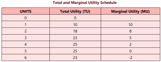
- Both TU and MU are interrelated.
TU = ∑ MU & MU = TUn – TUn-1 - At first unit, TU = MU.
- Initially, when TU is increasing at decreasing rate, MU is decreasing but remains positive.
- When TU is maximum and constant, MU = 0 (zero).
- When TU starts decreasing, MU becomes negative.
Law of Diminishing Marginal Utility
The law of diminishing marginal utility is founded on the key idea that, while a person's total wants are virtually limitless, each individual want can be satisfied. As a result, as a consumer increases their consumption of a good, the intensity of their desire for that good decreases, eventually reaching a point where they no longer wish to consume it. In simpler terms, it indicates that as a consumer consumes more units of a good, the additional satisfaction gained from each extra unit diminishes. It's important to highlight that it is the marginal utility, not the total utility, that decreases with increased consumption of a good.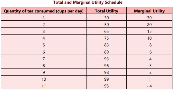
Let us illustrate the law with the help of an example. Consider table in which we have presented the total utility and marginal utility derived by a person from cups of tea consumed per day. When one cup of tea is taken per day, the total utility derived by the person is 30 utils (unit of utility) and marginal utility derived is also 30 utils with the consumption of 2nd cup per day the total utility rises to 50 but marginal utility falls to 20.
However, when the cups of tea consumed per day increases to 11, then instead of giving positive marginal utility, the eleventh cup gives negative marginal utility because it may cause him sickness.
The law of diminishing marginal utility is applicable only under certain assumptions:
(i) The different units consumed should be identical in all respects. The habit, taste, treatment and income of the consumer also remain unchanged.
(ii) The different units consumed should consist of standard units. If a thirsty man is given water by successive spoonful, the utility of second spoonful may conceivably be greater than the utility of the first.
(iii) There should be no time gap or interval between the consumption of one unit and another unit i.e. there should be continuous consumption.
(iv) The law may not apply to articles like gold, cash where a greater quantity may increase the lust for it.
(v) The shape of the utility curve may be affected by the presence or absence of articles which are substitutes or complements.
Consumer Surplus
The concept of consumer surplus was introduced by Alfred Marshall. It is a measure of the welfare that individuals derive from consuming goods and services, reflecting the benefits buyers receive from engaging in a market. This concept is significant not only in economic theory but also in government economic policies and business decision-making.Consumer demand for a commodity is influenced by the utility derived from that commodity. A consumer who derives greater utility from a good is willing to pay a higher price, and conversely, one who derives less utility will pay less. Each consumer's willingness to pay, based on their perceived utility, shapes the demand curve. When the price is less than or equal to what a consumer is willing to pay, the consumer is likely to purchase the good.
It is well-known that consumers often are willing to pay more for certain goods than the actual price they pay. This additional satisfaction gained from purchasing a good is referred to as consumer surplus, as defined by Alfred Marshall. Consumer surplus is defined as the difference between the total amount consumers are willing and able to pay for a good or service (as indicated by the demand curve) and the total amount they actually pay (i.e., the market price).
Marshall described consumer surplus as the “excess of the price which a consumer would be willing to pay rather than go without a thing over that which he actually does pay.” Therefore, consumer surplus can be expressed as:
Consumer Surplus = Willingness to Pay - Actual Payment.
This concept originates from the law of diminishing marginal utility. According to this law, as individuals acquire more of a good, the marginal utility it provides decreases. A consumer reaches equilibrium when the marginal utility of a good equals its price, meaning they buy a quantity of the good at which the marginal utility matches the price (assuming perfect competition in the market). Since the price remains constant for all units purchased, the consumer gains additional utility from all units consumed, except for the last one. This additional utility or surplus is termed consumer surplus.
Consider Table 7 in which we have illustrated the measurement of consumer surplus in case of commodity X. There is only one price for a commodity in the market at a particular point of time. The price of X is assumed to be ₹ 20.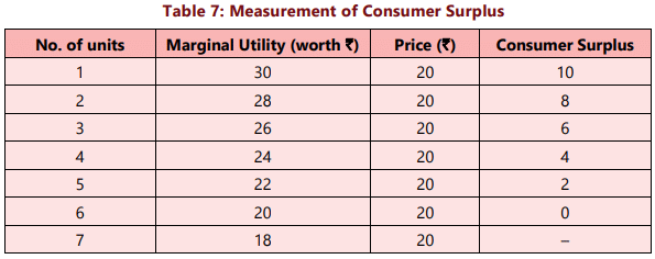
From the aforementioned table, we observe that when a consumer's consumption rises from 1 to 2 units, the marginal utility decreases from 30 to 28. As the consumer continues to increase consumption of good X, the marginal utility continues to diminish. Since the marginal utility of a unit of a good indicates the price the consumer is willing to pay, and assuming the market price is ₹20, the consumer achieves a surplus on every unit purchased up to the 6th unit. For instance, when purchasing 1 unit of X, the marginal utility is valued at ₹30 while the fixed price is ₹20, resulting in a surplus of ₹10. Similarly, when purchasing 2 units of X, the surplus is ₹8 [28 – 20]. This pattern continues, yielding consumer surpluses of 6, 4, and 2 for the 3rd, 4th, and 5th units, respectively. Upon purchasing the 6th unit, the consumer reaches equilibrium as the marginal utility equals the market price, resulting in no surplus. Thus, given the price of ₹20 per unit, the total surplus for the consumer amounts to 10 + 8 + 6 + 4 + 2 + 0 = ₹30.
The concept of consumer surplus is closely tied to the demand curve of a product, which reflects the buyer's willingness to pay and can also be utilized to gauge consumer surplus. The height of the demand curve represents the value that buyers assign to the good as evidenced by their willingness to pay. The disparity between the willingness to pay and the market price constitutes each buyer's consumer surplus. The difference between the willingness to pay and the actual price paid represents the net gain for the consumer, known as individual consumer surplus.
The total consumer surplus in a market, which is the aggregate of all individual consumer surpluses, equates to the area below the market demand curve but above the price. The term 'consumer surplus' often refers to both individual and total consumer surplus.
Consequently, the total area beneath the demand curve and above the price signifies the sum of the consumer surplus for all buyers in the market.
This concept of consumer surplus can be illustrated graphically. In the relevant figure, the X-axis represents the quantity of the commodity, while the Y-axis represents both marginal utility and the price of the commodity. The marginal utility (MU) curve slopes downward, indicating that as the consumer purchases more units of the commodity, the marginal utility declines. Marginal utility reflects the price a consumer is willing to pay for various units rather than forgo them. If OP is the prevailing market price, the consumer achieves equilibrium upon purchasing OQ units of the commodity, where the marginal utility equals the given price OP. The last unit, the Qth unit, does not generate any consumer surplus, as the price paid matches the marginal utility of that unit. For all units prior to the Qth unit, the marginal utility exceeds the price, resulting in a consumer surplus for those units.
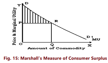
In Figure 15, the total utility is equal to the area under the marginal utility curve up to point Q i.e. ODRQ. But, given the price equal to OP, the consumer actually pays OPRQ. The consumer derives extra utility equal to DPR which is nothing but consumer surplus. (The portion of demand curve RD1 is not relevant for our consumer as MUx is less than Px in this part and therefore, the consumer will not buy any quantity beyond Q.)
The consumer welfare derived from a good is the benefit a consumer gets from consuming that good minus what the consumer paid to buy the good. Consumer surplus is the buyer's net gain from purchasing a good. Graphically, it is the triangular area below the demand curve and above the price line. The size of the consumer surplus triangle depends on the price of the good. A rise in the price of a good reduces consumer surplus; a fall in the price increases consumer surplus. Thus, a higher price results in a smaller consumer surplus and a lower price generates a larger consumer surplus. The change in consumer surplus on account of a fall in price can be illustrated with the help of figure16.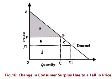
A fall in price from P to P1 increases consumer surplus from APE to A P1F.The increase in consumer surplus has two components.
(a) The increase in consumer surplus of existing buyers who were earlier paying price P (the rectangle marked b).
(b) The consumer surplus now available to the new buyers who started buying the commodity due to lower prices (the triangle c)
Applications
The concept of consumer surplus has significant practical applications. Here are a few:
- Consumer surplus measures the welfare that individuals gain from consuming goods and services. It is crucial for businesses to understand the level of consumer surplus enjoyed by various customer segments, as consumers who perceive a large surplus are more inclined to make repeat purchases.
- Understanding the nature and extent of surplus aids business managers in making informed pricing decisions. If a business can identify consumer groups with varying demand elasticity and those willing to pay higher prices for the same products, it can effectively implement price discrimination.
- Large-scale investment decisions require cost-benefit analyses that consider the potential consumer surplus generated by projects.
- Knowledge of consumer surplus is vital when a firm contemplates increasing product prices. Customers who experience minimal surplus may not be willing to purchase products at elevated prices, leading to reduced sales if prices are raised.
- Consumer surplus often guides finance ministers in determining which products to tax and the extent of tax increases. It is preferable to impose taxes or raise tax rates on commodities with high consumer surplus, as the welfare loss to citizens will be minimal.
Limitations
- It is frequently claimed that the notion of consumer surplus is theoretical and misleading. In practical scenarios, surplus satisfaction is challenging to quantify accurately.
- Consumer surplus cannot be precisely quantified due to the difficulty in measuring the marginal utilities of different units of a product consumed by an individual. In the case of essential goods, the marginal utilities of the initial units are infinitely large, resulting in an infinite consumer surplus.
- The consumer surplus associated with a product is influenced by the availability of substitutes. There is no straightforward method for determining the utility scale of items used for their prestige value (e.g., diamonds).
- Furthermore, consumer surplus cannot be expressed in monetary terms because the marginal utility of money fluctuates as purchases occur and the consumer's money supply decreases. (Marshall posited that the marginal utility of money remains constant, but this assumption is unrealistic).
- The concept can only be accepted under the assumption that utility can be quantified in monetary terms or otherwise. Many contemporary economists argue that this is not feasible.
Indifference Curve Analysis
In the previous section, we examined the marginal utility analysis of demand. An alternative and more realistic method for explaining consumer demand is the ordinal utility approach. This method employs the indifference curve to analyze consumer behavior and is centered around consumer preferences. It operates on the premise that human satisfaction, being a psychological phenomenon, cannot be quantified in monetary terms as attempted in Marshall’s utility analysis. Thus, it is scientifically more valid to rank preferences rather than to measure them monetarily. Consequently, the consumer preference approach is an ordinal concept that focuses on the ranking of preferences, in contrast to Marshall’s cardinality approach.Assumptions Underlying Indifference Curve Approach
(i) The basis of consumer behavior theory is the premise that consumers are aware of their own tastes and preferences and have complete information regarding all relevant aspects of their economic environment.
(ii) Consumers are viewed as rational beings who engage in rational behaviors that lead to choosing a more desirable consumption bundle over a less desirable one.
(iii) Indifference curve analysis posits that utility can only be expressed ordinally. Consumers can rank all possible combinations of goods based on the satisfaction they provide. For instance, if presented with combinations A, B, C, D, and E, they can order them by preference, but if they prefer A to B, they cannot quantify how much more they prefer A over B.
(iv) Consumer preferences are assumed to be transitive. If a consumer favors combination A over B, and B over C, then they must also favor combination A over C, indicating a consistent consumption pattern.
(v) If combination A contains more goods than combination B, then A is assumed to be preferred to B. This is often referred to as the "more is better" assumption or the non-satiation assumption.
Indifference Curves
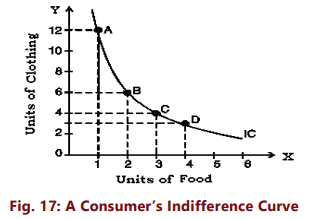
The ordinal analysis of demand, as discussed by Hicks and Allen, utilizes indifference curves to graphically represent consumer preferences. An indifference curve illustrates all combinations of two goods that provide the same level of satisfaction to the consumer. Since every combination on an indifference curve yields equal satisfaction, the consumer remains indifferent among them. Essentially, it depicts the set of all bundles of goods that the consumer considers equally desirable. In other words, since all combinations deliver the same level of satisfaction, the consumer prefers them equally and is indifferent about which combination they receive. An indifference curve is also referred to as an iso-utility curve or equal utility curve.To understand indifference curves, let us consider the example of a consumer who has one unit of food and 12 units of clothing. Now, we ask the consumer how many units of clothing he is prepared to give up to get an additional unit of food, so that his level of satisfaction does not change. Suppose the consumer says that he is ready to give up 6 units of clothing to get an additional unit of food. We will have then two combinations of food and clothing giving equal satisfaction to the consumer: Combination A which has 1 unit of food and 12 units of clothing, and combination B which has 2 units of food and 6 units of clothing. Similarly, by asking the consumer further how much of clothing he will be prepared to forgo for successive increments in his stock of food so that his level of satisfaction remains unaltered, we get various combinations as given in table 8:

Now, if we plot the above schedule, we will get the following figure. In Figure 17, an indifference curve IC is drawn by plotting the various combinations given in the indifference schedule. The quantity of food is measured on the X axis and the quantity of clothing on the Y axis. As in indifference schedule, the combinations lying on an indifference curve will give the consumer the same level of satisfaction.
Indifference Curve Map
The utility function of an individual can be illustrated using an indifference curve map, which comprises multiple indifference curves, each representing a distinct level of satisfaction. In essence, a collection of indifference curves is referred to as an indifference curve map. Every indifference curve consists of points that all reflect the same utility level. Combinations of goods located on indifference curves that are farther from the origin are deemed more desirable than those on curves that are closer to the origin. Transitioning upwards and to the right from one indifference curve to another indicates an increase in utility, while moving downwards and to the left signifies a decrease. Hence, an indifference curve map effectively portrays the comprehensive view of consumer preferences and tastes.
In Figure 18, a consumer's indifference curve map is presented, featuring three distinct indifference curves.
We have marked good X on X-axis and good Y on Y-axis. It should be noted that while the consumer is indifferent among the combinations lying on the same indifference curve, he certainly prefers the combinations on the higher indifference curve to the combinations lying on a lower indifference curve because a higher indifference curve signifies a higher level of satisfaction. Thus, while all combinations of IC1 give him the same satisfaction, all combinations lying on IC2 give him greater satisfaction than those lying on IC1.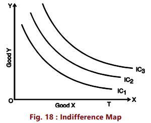
Marginal Rate of Substitution
The Marginal Rate of Substitution (MRS) indicates the rate at which a consumer is willing to trade off goods X and Y while maintaining the same level of satisfaction (i.e., moving along an indifference curve).
The MRS along any section of an indifference curve represents the highest rate at which a consumer would willingly exchange units of Y for units of X. The MRS at any point on the curve equals the (absolute value of) the slope at that specific point. When assessed at a point, the MRSxy indicates the maximum rate at which a consumer would trade good Y for a very small increase in good X.
For example, consider Table-8. Initially, the consumer consumes 1 unit of food and 12 units of clothing. Then, he gives up 6 units of clothing to gain an additional unit of food, keeping his satisfaction level unchanged. Here, the MRS is 6. Similarly, when moving from B to C and from C to D in his indifference schedule, the MRS values are 2 and 1, respectively. Therefore, we can define the MRS of X for Y as the quantity of Y that can be sacrificed to offset the gain of one unit of X while keeping the satisfaction level constant.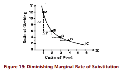
We observe that the Marginal Rate of Substitution (MRS) is decreasing; as a consumer acquires more units of food, the trade-off or substitution rate diminishes, meaning they are willing to give up fewer units of clothing. (Refer to Figure 19). As a consumer moves down their indifference curve, they gain utility from consuming additional units of good X, but lose an equivalent amount of utility from reduced consumption of good Y. However, the utility levels at which the consumer starts differ at each point. At point A in Figure 19, the consumer has a small quantity of food, resulting in a high marginal utility for food at that point. Therefore, an additional unit of food significantly increases their total utility. Conversely, the consumer already consumes a large amount of clothing, leading to a low marginal utility for clothing at this point. This indicates that a substantial decrease in clothing consumption is necessary to offset the increased utility from the extra unit of food.
In contrast, at point C, the consumer has a much larger quantity of food and a smaller quantity of clothing compared to point A. This implies that an additional unit of food adds less utility, while the cost of forgoing a unit of clothing results in a greater loss of utility than at point A. Consequently, the consumer is inclined to give up fewer units of clothing for an additional unit of food at point C (they sacrifice only 2 units of clothing for 1 unit of food, compared to 6 units of clothing at point A for one unit of food).
Moving down the indifference curve—reducing clothing consumption while increasing food consumption—will yield two opposing effects on the consumer’s total utility: a decline in total utility due to lower clothing consumption and an increase in total utility from higher food consumption. To maintain constant satisfaction levels, these two effects must perfectly offset each other as the consumer descends the indifference curve. The principle of diminishing marginal rate of substitution states that the more of good Y a person consumes relative to good X, the less willing they become to substitute an additional unit of X for Y.
There are two reasons for this:
- The desire for a specific good is satiable; hence, as a consumer obtains more of it, their intensity of desire for additional units decreases. In this example, as the consumer acquires more food, their eagerness for more food diminishes.
- Most goods are imperfect substitutes for one another. If they could perfectly substitute each other, the MRS would remain constant.
We know that along the indifference curve:
(Change in total utility due to lower clothing consumption) = (Change in total utility due to higher food consumption)
Change in total utility due to a change in clothing consumption = MU c × ΔQ c
Change in total utility due to a change in food consumption = MUf× ΔQf
Therefore, along the indifference curve:−MUc × ΔQc = MUf× ΔQf
Note that the left-hand side of the equation has a minus sign as it represents the loss in total utility from decreased clothing consumption. This must equal the gain in total utility from increased food consumption, represented by the right-hand side of the equation. Along the indifference curve:
To generalize, the marginal rate of substitution of X for Y (MRSxy) is the slope of the indifference curve.
As the number of units of Y the consumer is willing to sacrifice gets lesser and lesser, the marginal rate of substitution gets smaller and smaller as we move down and to the right along an indifference curve. That is, the indifference curve becomes flatter (less sloped) as we move down and to the right.
Properties of Indifference Curves
The following are the main characteristics or properties of indifference curves:- Indifference curves slope downward to the right: This characteristic indicates that the two goods can substitute for one another; as the quantity of one good in the combination increases, the quantity of the other good decreases. This is crucial for maintaining the same level of satisfaction along an indifference curve.
- Indifference curves are always convex to the origin: It has been noted that as a consumer substitutes more of one good (X) for another (Y), they are willing to give up less and less of the good being substituted (Y). This phenomenon is referred to as the diminishing marginal rate of substitution. For instance, in the case of food and clothing, as a consumer acquires more food, they are willing to forgo fewer units of clothing. This behavior occurs because the desire for a specific good becomes satiated; as a person has more of a good, their intensity of desire for that good diminishes. In other words, the perceived value of an additional unit of one good decreases more rapidly compared to the other good whose quantity is declining. This diminishing marginal rate of substitution results in the convex shape of the indifference curves.
However, there are two extreme situations.
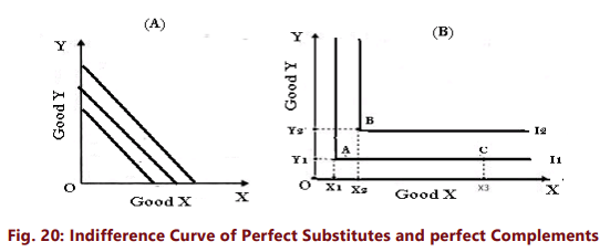
- When two goods are perfect substitutes of each other, the consumer is completely indifferent as to which to consume and is willing to exchange one unit of X for one unit of Y. His indifference curves for these two goods are therefore straight, parallel lines with a constant slope along the curve, or the indifference curve has a constant MRS.[Figure 20(A)].
- Goods are perfect complements when a consumer is interested in consuming these only in fixed proportions. When two goods are perfect complementary goods (e.g. left shoe and right shoe), the consumer consumes only bundles like A and B in figure 20(B) in which both X and Y in equal proportions. With a bundle like A or B, he will not substitute X for Y because an extra piece of the other good (here a single shoe) is worthless for him. The reason is that neither an additional left shoe nor a right shoe without a paired one of each, adds to his total utility. In such a case, the indifference curve will consist of two straight lines with a right angle bent which is convex to the origin, or in other words, it will be L shaped. [Figure 20(B)] Avery interesting fact about this is that in the case of perfect complements, the marginal rate of substitution is undefined because an individual’s preferences do not allow any substitution between goods.

(iii) Indifference curves can never intersect each other: No two indifference curves will intersect each other although it is not necessary that they are parallel to each other. In case of intersection the relationship becomes logically absurd because it would show that higher and lower levels are equal, which is not possible. This property will be clear from Figure 21.
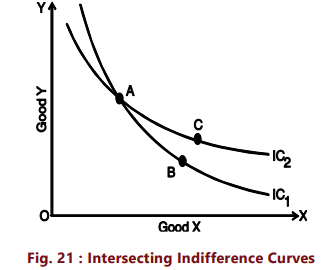
In figure 21, IC1 and IC2 intersect at A. Since A and B lie on IC1 , they give same satisfaction to the consumer. Similarly since A and C lie on IC2, they give same satisfaction to the consumer. This implies that combination B and C are equal in terms of satisfaction. But a glance will show that this is an absurd conclusion because certainly combination C is better than combination B because it contains more units of commodities X and Y. Thus we see that no two indifference curves can touch or cut each other.
(iv) A higher indifference curve represents a higher level of satisfaction than the lower indifference curve: This is because combinations lying on a higher indifference curve contain more of either one or both goods and more goods are preferred to less of them.
(v) Indifference curve will not touch either axes: Another characteristic feature of indifference curve is that it will not touch the X axis or Y axis. This is born out of our assumption that the consumer is considering different combination of two commodities. If an indifference curve touches the Y axis at a point P as shown in the figure 22, it means that the consumer is satisfied with OP units of Y commodity and zero units of X commodity. This is contrary to our assumption that the consumer wants both commodities although in smaller or larger quantities. Therefore an indifference curve will not touch either the X axis or Y axis.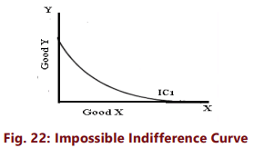
The Budget Line
From the analysis of ordinal utility, we have gained insight into one aspect of consumer behavior: consumer preferences. A higher indifference curve represents a greater level of satisfaction compared to a lower one. Consequently, consumers aim to achieve the highest indifference curve possible to maximize their satisfaction. However, in their pursuit of acquiring more goods and increasing satisfaction, they face two constraints: first, they must pay for the goods, and second, they have a limited income to spend on purchases.
Consumers strive to optimize their well-being while adhering to these constraints. The primary constraint that individuals encounter when deciding on consumption is the budget constraint. This means that consumers typically operate with a limited income, which restricts their consumption capacity. As established, a consumer's total spending on goods and services can be less than their budget constraint, but it cannot exceed it.
Algebraically, we can write the budget constraint for two goods X and Y as:
PXQX + PYQY ≤ B
Where
PX and PY are the prices of goods X and Y and QX and QY are the quantities of goods X and Y chosen and B is the total money available to the consumer.
The requirement illustrated by the equation above that a consumer must choose a consumption bundle that costs no more than his or her income is known as the consumer’s budget constraint. A consumer’s consumption possibilities are the set of all consumption bundles that can be consumed given the consumer’s income and prevailing prices. We assume that the consumer in our analysis uses up his entire nominal money income to purchase the commodities. So that his budget constraint is PXQX + PYQY = B
The following table shows the combinations of Ice cream and chocolates a consumer can buy spending the entire fixed money income of ₹100, with the prices ₹ 20 and ₹10 respectively.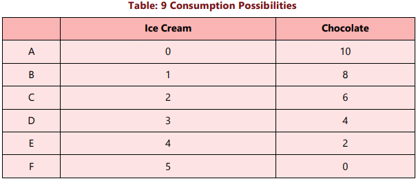
The budget constraint can be explained by the budget line or price line. In simple words, a budget line shows all those combinations of two goods which the consumer can buy spending his given money income on the two goods at their given prices. All those combinations which are within the reach of the consumer (assuming that he spends all his money income) will lie on the budget line. The consumer could, of course, buy any bundle that cost less than ₹ 100.(e.g. Point K)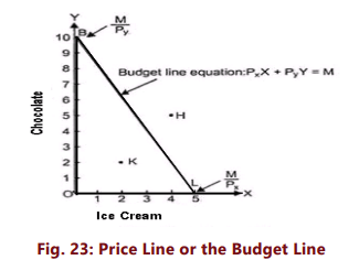
It should be noted that any point outside the given price line, say H, will be beyond the reach of the consumer and any combination lying within the line, say K, shows under spending by the consumer. The slope of the budget line is determined by the relative prices of the two goods. It is equal to ‘Price Ratio’ of two goods i.e. PX /PY i.e. It measures the rate at which the consumer can trade one good for the other. The budget line will shift when there is:
- A change in the prices of one or both products with the nominal income of the buyer (budget) remaining the same.
- A change in the level of nominal income of the consumer with the relative prices of the two goods remaining the same.
- A change in both income and relative prices
Consumer Equilibrium
Having described indifference curves and the budget line, we can now clarify how a consumer attains equilibrium by selecting the optimal consumption bundle while considering constraints. A consumer reaches equilibrium when maximizing satisfaction from goods, making rearrangement of purchases unnecessary. We assume that:
- The consumer possesses a defined indifference map that illustrates preferences for various combinations of two goods, X and Y.
- The consumer has a fixed income that must be entirely spent on goods X and Y.
- The prices of goods X and Y are predetermined and unchanging.
- All goods are uniform and can be divided.
- The consumer behaves 'rationally' to maximize satisfaction.
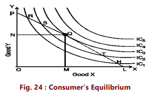
To show which combination of two goods X and Y the consumer will buy to be in equilibrium we bring his indifference map and budget line together.
The indifference map illustrates a consumer's preference between different combinations of two goods, while the budget line represents the combinations that can be purchased with the consumer's income and the prices of those goods. In Figure 24, curves IC1, IC2, IC3, IC4, and IC5 are displayed alongside budget line PL for goods X and Y. Each combination on budget line PL has the same cost, meaning combinations R, S, Q, T, and H have identical prices for the consumer. The consumer's goal is to maximize satisfaction, aiming to reach the highest possible indifference curve.
Given the budget constraint, the consumer must select combinations solely from those located on the budget line. What combination will our theoretical consumer select? The optimal choice for a consumer must fulfill two conditions:
- It will be located on the budget line.
- It will aim to reach the highest indifference curve possible.
- It will lie on the highest indifference curve possible
The consumer can arrive this choice moving down his budget line starting from point R. While doing this, he will pass through a variety of indifference curves (To make the diagram simple, we have drawn only a few). Suppose he chooses R. We see that R lies on a lower indifference curve IC1, when he can very well afford S, Q or T lying on higher indifference curves. Similar is the case for other combinations on IC1 , like H. Again, suppose he chooses combination S (or T) lying on IC2. But here again we see that the consumer can still reach a higher level of satisfaction remaining within his budget constraints i.e., he can afford to have combination Q lying on IC3 because it lies on his budget line. Now, what if he chooses combination Q? We find that this is the best choice because this combination lies not only on his budget line but also puts him on the highest possible indifference curve i.e., IC3. The consumer can very well wish to reach IC4 or IC5, but these indifference curves are beyond his reach given his money income. Thus, the consumer will be at equilibrium at point Q on IC3. What do we notice at point Q? We notice that at this point, his budget line PL is tangent to the indifference curve IC3. In this equilibrium position (at Q), the consumer will buy OM of X and ON of Y. At the tangency point Q, the slopes of the price line PL and the indifference curve IC3 are equal. The slope of the indifference curve shows the marginal rate of substitution of X for Y (MRSxy) which is equal to  while the slope of the price line indicates the ratio between the prices of two goods i.e.
At equilibrium point Q,
Thus, we can say that the consumer is in equilibrium position when the price line is tangent to the indifference curve or when the marginal rate of substitution of goods X and Y is equal to the ratio between the prices of the two goods. We have seen that the consumer attains equilibrium at the point where the budget line is tangent to the indifference curve and
In fact the slope of the indifference curve points to the rate at which the consumer is willing to give up good Y for good X. The slope of the budget line tells us the rate at which the consumer is actually able to trade good X and good Y. When both these are equal, he will be maximizing his satisfaction given the constraints. The indifference curve analysis is superior to utility analysis: (i) it dispenses with the assumption of measurability of utility (ii) it studies more than one commodity at a time (iii) it does not assume constancy of marginal utility of money (iv) it segregates income effect from substitution effect.
Summary
- The existence of human wants is the foundation for all economic activities in society. All desires, tastes, and motives of individuals are referred to as wants in Economics. In this context, wants are categorized into necessaries, comforts, and luxuries.
- Utility indicates the want-satisfying ability of goods and services. It is not an absolute measure but rather relative. This concept is subjective and varies based on individual mental attitudes.
- Two significant theories of utility are cardinal utility analysis and ordinal utility analysis. The law of diminishing marginal utility states that as a consumer consumes more of a commodity, each additional unit provides less satisfaction.
- Consumer surplus represents the difference between the price a consumer is willing to pay for a commodity and the actual price paid. It reflects the buyer's net benefit from purchasing a good. Graphically, it is depicted as the triangular area below the demand curve and above the price line. An increase in the price of a good decreases consumer surplus, while a decrease in price increases it.
- The indifference curve theory, an ordinal theory, illustrates a household’s preferences among different bundles of goods through indifference curves. The marginal rate of substitution indicates the rate at which a consumer is willing to exchange goods X and Y.
- Key properties of an indifference curve include: it slopes downward to the right, is always convex to the origin, no two indifference curves intersect, it does not touch the axes, and a higher indifference curve represents a higher level of satisfaction.
- When two goods are perfect substitutes, their indifference curves are straight, parallel lines with a constant slope, indicating a constant marginal rate of substitution. Conversely, goods are perfect complements when a consumer prefers to consume them in fixed proportions, resulting in L-shaped indifference curves that are convex to the origin.
- The budget line or price line illustrates all combinations of two goods that a consumer can purchase with their given income at specified prices. The slope of the budget line is determined by the relative prices of the two goods, expressed as the price ratio (PX/PY), which indicates the rate at which one good can be traded for another.
- The budget line shifts when there is a change in the price of one or both goods while keeping the consumer's nominal income constant, or when there is a change in the consumer’s nominal income while relative prices remain unchanged.
- A consumer is considered to be in equilibrium when they achieve maximum satisfaction from their goods and cannot rearrange their purchases for better satisfaction. Consumer equilibrium occurs at the point where the budget line is tangent to the indifference curve, fulfilling the condition MUx / Px = MUy / Py = MUz / Pz.
|
124 videos|191 docs|88 tests
|
FAQs on Unit 2: Theory of Consumer Behaviour Chapter Notes - Business Economics for CA Foundation
| 1. What are the different classifications of human wants in economics? |  |
| 2. How does Total Utility (TU) relate to Marginal Utility (MU)? |  |
| 3. What is the Law of Diminishing Marginal Utility? |  |
| 4. What is Consumer Surplus and why is it important? |  |
| 5. How does Indifference Curve Analysis help in understanding consumer preferences? |  |
|
124 videos|191 docs|88 tests
|

|
Explore Courses for CA Foundation exam
|

|
