Fatigue strength and the S-N diagram | Design of Machine Elements - Mechanical Engineering PDF Download

Fatigue Failure

Fatigue failure occurs when materials fail under fluctuating stresses that are lower than the material's ultimate tensile strength, and sometimes even lower than its yield strength. Observations have shown that the resistance to these stresses decreases as the number of stress cycles increases. This phenomenon, where materials exhibit reduced resistance to fluctuating stresses over time, is known as fatigue.

Difference Between Static Load Failure and Fatigue Failure

There is a fundamental difference between failure due to static load and failure due to fatigue.

Static Load Failure

• Illustration: This type of failure is exemplified by the simple tension test.
• Load Application: The load is applied gradually, providing sufficient time for the material's fibers to elongate.
• Material Behavior: In ductile materials, there is significant plastic deformation before fracture.
• Fracture Surface: The resulting fracture surface has a silky, fibrous structure due to the stretching of crystals.

Fatigue Failure

• Initiation: Fatigue failure begins with a crack at a specific point in the material.
• Likely Regions for Cracks:
  • Regions of discontinuity such as oil holes, keyways, and screw threads.
  • Regions with irregularities from machining operations, such as surface scratches, stamp marks, and inspection marks.
  • Internal cracks due to material defects like blow holes.

These regions experience stress concentrations due to the initial crack. Under fluctuating stresses, the crack propagates until the cross-sectional area of the component is significantly reduced, leading to sudden fracture.

Characteristics of Fatigue Failure

1. Slow Crack Growth: This region shows a fine fibrous appearance, indicating the gradual progression of the crack.
2. Sudden Fracture: This region exhibits a coarse granular appearance, marking the final, abrupt failure of the material.

Understanding these differences is crucial for designing components that can withstand both static and fluctuating loads, thereby preventing premature failures.

Endurance Limit 

The fatigue or endurance limit for a material is defined as the maximum value of completely reversing stress that the standard specimen can sustain for an unlimited number of cycles without fatigue failure. The endurance limit, denoted as σe’, is considered as a criterion of failure under fluctuating stresses. In laboratory, the endurance limit is determined by means of a rotating beam machine. It was developed by R. R, Moore. The results of the tests are plotted by means of an S−N curve. The S−N curve is a graphical representation of the maximum applied stress σf versus the number of stress cycles N before the fatigue failure on a log−log paper as shown in the figure.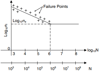
 Each test gives one failure point on the S−N curve. In practice, the points are scattered on the figure and an average curve is drawn through them. For ferrous materials like steels, the S−N curve becomes asymptotic at 106 cycles, which indicate the stress level corresponding to the infinite number of stress cycles. The magnitude of this stress is called the “endurance strength” of the material.
The S−N curve shown in figure is valid only for ferrous materials. For non ferrous materials, the S−N curve slopes gradually even after 106 cycles. Theses materials do not have a limiting value of endurance strength in a true sense. In this case, the endurance limits stress is always expressed as a function of the number of stress cycles. The endurance stress in a true sense, is not exactly a property of the material, like ultimate or yield strengths. It is affected by the size and shape of the components the surface finish, temperature and the notch sensitivity of the material. 

Notch Sensitivity

It is observed that the actual reduction in the endurance strength of a material due to stress concentration is less than the amount indicated by the theoretical stress concentration factor K_t. Two separate notations − K_t and K_f are therefore used for stress concentration factors. K_t is the theoretical stress concentration factor, K_f is the fatigue stress concentration factor, which is defined as follows : 

This factor K_f is applicable to actual materials and depends upon the grain size of the material. It is observed that there is a greater reduction in the endurance strength of fine grained material, as compared to coarse grained materials, due to stress concentration. Notch sensitivity is defined as the susceptibility of a material to succumb to the damaging effects of the stress raising notches in fatigue loading. The notch sensitivity factor q is defined as;

where σ0 is the nominal stress as obtained by elementary equations. The above equation is rearranged in the following form :
K_f = 1 + q(K_t − 1) (* K_t depends upon d/w ratio)

Estimation of Endurance limit 

There is an approximate relationship between the endurance strength and the ultimate tensile strength of the materials. For Steels,
σ_e′ = 0.5 σ_ut 
For cast iron and cast steels
σ_e′ = 0.4 σ_ut 
* σ_e′ is the endurance limit stress for a rotating beam specimen subjected to reversed bending stress whereas σe is the endurance limit stress for a particular mechanical component subjected to reversed bending stress. These relationships are based on 50% reliability. The endurance strength of a component is different from the endurance strength of a rotating beam specimen due to a number of factors. The difference arises due to the fact that there are standard specifications and working conditions for the rotating beam specimen, while the actual components works under different conditions. Different modifying factors are used in practice to account for these conditions. The relationship between σ_e and σ_e′ is as follows :
 σ_e = k_a k_b k_c k_d σ_e 
where k_a = surface finish factor k_b = size factor k_c = reliability factor k_d = modifying factor to account for stress concentration When the surface finish is poor, the endurance strength is reduced because of scratches. The variation in surface finish between the specimen and the component is accounted by the surface finish factor(* k_a is related to σ_ut). The size factor kb depends upon the size of the cross section of the component. As the size of the component increases, the surface area also increases, resulting in a greater number of surface defects. The endurance strength, therefore, reduces with increasing size of the components. The reliability factor k_c depends upon the reliability that is considered in the design of the component. The reliability of the fatigue test is 50%.
The modifying factor k_d to account for the effect of stress concentration is defined as
kd = 1 /  K
The endurance strength (τe) of a component subjected to fluctuating torsional shear stresses is obtained from the endurance strength in reversed bending (σe) using theories of failure.
According to the maximum shear stress theory,

 According to distortion energy theory

Types of Fatigue Design Problems

There are two types of problems in fatigue design :
(i) Components subjected to completely reversed stresses
(ii) Components subjected to fluctuating stresses
The mean stress is zero in case of completely reversed stresses. The stress distribution consists of tensile stresses for the first half cycle and compressive stresses for the remaining half cycle and the stress cycle passes through zero. In case of fluctuating stresses, there is always a mean stress, and the stresses can be purely tensile, purely compressive or mixed depending upon the magnitude of the mean stress. Such problems are solved with the help of Gerber, Goodmann or Soderberg equations. The design problems for completely reversing stresses are further divided into two groups, i) design for infinite life, and ii) design for finite life. When the component is to be designed for infinite life, the endurance limit becomes the criterion of failure. The stresses induced in such components should be lower than the endurance limit in order, to withstand the infinite number of cycles. Such components are designed with the help of following equations :

where σ_a and τa are induced stresses or stress amplitudes in the component and σ_e and τ_e are corrected endurance strengths in reversed bending and torsion respectively. When the component is to be designed for finite life, the S−N curve can be used.  

Cumulative Fatigue Damage

In certain applications, the mechanical component is subjected to different stress levels for different parts of the work cycle. The life of such a component is determined by Miner’s equation. Let a component is subjected to completely reversed stresses σ₁ for n₁ cycles, σ₂ for n₂ cycles and so on. Let N₁ be the number of stress σ₁ is acting. One stress cycle will consume (1/N₁) of the fatigue life and since there are n₁ such cycles at this stress level, the proportionate damage of fatigue life will be (1/N₁)n₁ or (n₁/ N₁). Similarly, the proportionate damage at stress level σ₂ will be (n₂ / N₂). Adding these quantities we get,

The above equation is known as Miner’s equation. Sometimes, the number of cycles n₁, n₂ … at stress levels σ₁, σ₂, … are unknown. Suppose that α₁, α₂ ,… are proportions of the total life that will be consumed by the stress levels σ₁ , σ₂ etc. Let N be the total life of the component. Then  

Substituting these values in Miner’s equation, 

Also α₁ + α₂ + … α_x = 1. With the help of these equations, the life of the component subjected to different stress levels is determined.

Components Subjected To Fluctuating Stresses

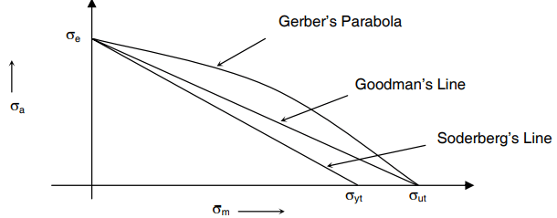
There are three methods for components subjected to fluctuating stress (mean stress is not zero)
(i) Gerber’s Parabola
(ii) Goodman’s Straight Line
(iii) Soderberg’s Straight Line Gerber’s Parabola
Gerber argued that te maximum value that stress amplitude σ_a, assume will be the fatigue strength in fully reversed stress cycle, σ_e. Similarly, the maximum value of mean stress σ_m, would be the ultimate tensile strength of the material σ_ut in the absence of any alternating stress. He further assumed that σ_a and σ_m will have a parabolic relationship. The relationship is expressed in the figure below and expressed as : 

This is obvious that when σa vanishes, i.e. when loading is only static;
σ_m = σ_a 
and when σm vanishes, i.e. when loading is only reversible
σ_a = σ_e (fatigue or endurance strength)
Gerber’s Parabola could be used to calculate fatigue strength, σ_a, when any static stress, σ_m, is super imposed upon fully reversed stress cycle.

Goodman’s Straight Line

Goodman’s relationship was more simplified. While allowing σ_a and σ_m to assume maximum values of σ_e and σut respectively, he correlated σ_a and σm by a straight line. It can be seen that for a given static superimposed stress, σ_m, this linear relationship predicts a lower effective fatigue strength than parabolic relation. Goodman’s line can be represented by following mathematical relation; 

It is obviously seen that
when σ_a = 0, σ_m = σ_ut (static loading) and
when σ_m = 0, σ_a = σ_e (only reversible loading)  

Soderberg’s Straight Line

Soderberg’s proposed that σ_m can assume a maximum value equal to the yield strength of the material σ_yt while maximum value of σ_a would still remain σ_e. He further assumed linear variation σ_a with respect to σ_m. It is also obvious that Soderberg’s proposition results in smaller value of σ_a for a given value of σ_m, as compared to other two proposals. Soderberg’s straight line is expressed as :

From this equation it is obvious that when
σ_a = 0, σ_m = σ_yt (static loading) and
when σ_m = 0, σ_a = σ_e (only reversible loading)

Experimental Evidence

The experimental results for ductile materials generally lie between Gerber’s parabola and Goodman’s Straight line, while for brittle materials the results mostly lie below Goodman’s line but bounded by an inverse of Gerber’s parabola on the lower side. Mathematically the experimental results seem to follow :

where
x = 1.6 for ductile material and
 x = 0.6 for brittle material.
The quantity in brackets can be regarded as fatigue strength reduction factor due to superimposed static stress.
Neither ductile nor brittle materials follow Soderberg’s relationship to any approximation. Secondly, Gerber’s parabola and Goodman’s Straight Line are followed only in the first quadrant, i.e. when both σ_a and σm are positive.
For negative values of σ_m , almost same value of σ_a can be applied on a ductile material as will be applicable for σ_m = 0.
 On the other hand for a brittle material, endurance limit, σ_a increases according to a linear law with decreasing values of σm beyond σ_m = 0.
Hypotheses of Goodman and Gerber are equally applicable to bending, axial and torsional loadings.  

 Note : It may be noted that Goodman’s Straight line results in lowest value of effective fatigue strength and it is generally followed for design purposes. 

Complex Fluctuating Stresses

If the state of stress at any point is described by  then the principal fluctuating stresses σ_p1 σ_p2 and can be calculated from the results the mean principal stresses σ_p1m and σ_p2m may be calculated. Similarly, the variable components of two principal stresses σ_p1 σ_p2 and may be calculated.
The distortion energy criterion is used to calculate equivalent mean and equivalent variable components of stresses if material is steel. If however, the material is cast iron, the equivalent mean and equivalent variable components are calculated by application of maximum principal stress criterion.
For example, if for steel,  and are equivalent Von Mises stresses (i.e. following distortion energy criterion), then;

For cast iron, if  and are equivalent principal stresses, then

Equivalent stress Method

Goodman’s equation may be rewritten as : 

The right hand side of this equation is named as equivalent direct or normal stress, denoted by σ_n. Thus 

 The equation may also be written for fluctuating shearing stress, and an equivalent shearing stress, can be defined in the same way. Call this equivalent shearing stress as τ_n, so that, 

 σ_n and τ_n are then treated as direct and shearing stress components acting at critical point and proper theory of failure may be applied using σn and τn for calculation of dimensions or factor of safety.

Practical Measures to Combat Fatigue

(i) Material Selection : The materials selected for machine elements should be perfectly homogeneous since cracks can often initiate and extend around large size impurities and inhomogeneities. Fine grained structure is also helpful because in such microstructures the grain boundaries largely act as barriers to cracks. As far as possible material should be free from internal stress raisers such as non metallic inclusions, cavities, cracks etc.
(ii) Stress Concentration : The sites of stress concentration that are intentionally introduced in machine parts to fulfill some purpose must be carefully planned so as to have minimum possible stress concentration factor. stress concentration factor of shoulder (a) in a shaft may be reduced by grooving circumferentially along the transition (b) or by providing a more generous groove on larger diameter region which would not interfere with the design requirements, (c) similarly a stress concentration due to circumferential groove, (d) may be relieved by two smaller grooves one on either side, (e) similar undercuts may be provided at the end of thread in a threaded member.
(iii) Machinery and Fabrication : Poor machining resulting into bad surface finish is may times the cause of fatigue failure. Surfaces should be finished smoothly without leaving a nick or blemish on the surface. Fabrication methods such as forging or welding may result into stress raisers. Welding joins need careful designing since they cause stress raisers.
(iv) Special Methods to Improve Fatigue Strengths : Mechanical working of surface whereby residual compressive stresses are generated on the surface are very helpful in improving fatigue behaviour. Hammer peening, shot peening or surface rolling are common treatments which are given to machine element surfaces particularly in the region of stress concentration. Surface strengthening may also be achieved through case hardening, nitriding, cyaniding, flame or induction hardening.

Solved Numericals

Q1. A cylindrical shaft is subjected to alternating stress of 100 MPa. Fatigue strength to sustain 1000 cycles is 490 MPa. If the corrected endurance strength is 70 MPa, What will be the estimated shaft life in revolutions? If the fatigue strength of the bar to withstand N cycles is 100 MPa then what will be the value of N (To the nearest integer)?
Ans: 281800 - 282000
The fatigue strength of the bar is calculated using the SN diagram where for 103 cycles the stress is 0.9Sut and for 106 cycles, the stress is endurance limit (S_e).

Calculation:
Given:
For σ = 100 MPa → N = ?
For 1000 cycle → σ = 490 MPa = 0.9 S_ut
The corrected endurance limit, S_e  = 70 MPa
At σ_e → N = 10⁶ cycle
Using the S - N curve for the equation of line AB,

$\frac{\log }{10}=\frac{6}{-}$
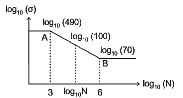
⇒ N = 281914 cycle

Q2. The figure shows the relationship between fatigue strength (S) and fatigue life (N) of a material. The fatigue strength of the material for a life of 1000 cycles is 450 MPa, while its fatigue strength for a life of 10⁶ cycles is 150 MPa.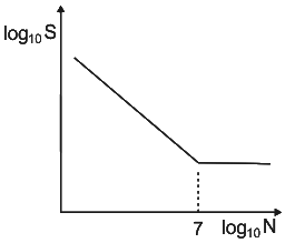 

The life of a cylindrical shaft made of this material subjected to an alternating stress of 200 MPa will then be ____________ cycles (round off to the nearest integer).
Ans: 152000 - 165000
Solution: 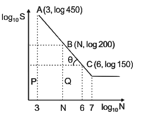In Δ APC

In Δ BQC

Calculation:
Given:
S₁ = 450 MPa, N₁ = 1000 cycles, S₂ = 150 MPa, N₂ = 10⁶ cycles.

6 - log N = 0.785578
log N = 5.214422
Number of cycle (N) equals 10^5.214422 = 163842 cycles.

Q3. A machine element has an ultimate strength (σ_u) of 600 N/mm², and endurance limit (σ_en) of 250 of 250 N/mm². The fatigue curve for the element on a log-log plot is shown below. If the element is to be designed for a finite life of 10000 cycles, the maximum amplitude of a completely reversed operating stress is_______N/mm².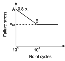Ans: 370 - 390
Solution:
Given: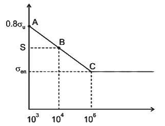  

σ_u = 600 N/mm²
σ_en = 250 N/mm²
Co-ordinates of points are:
A → (log (0.8σ_u), 3)
B → (log S, 4)
C → (log σ_en, 6)
Now Slope AB = Slope AC

S = 386.19

Q4. A cylindrical shaft is subjected to an alternating stress of 100 MPa. Fatigue strength to sustain 1000 cycle is 490 MPa. If the corrected endurance strength is 70 MPa, estimated shaft life will be
Solution:

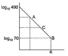Equation of straight line containing (3, log₁₀ 490) and (6, log₁₀ 70)

$\frac{𝑦}{-}=\frac{1.84}{-}$y – 1.84 = -0.28 (x – 6)
At y = log₁₀ (100) = 2
⇒ 2 – 1.84 = - 0.28 (x – 6)
x = 5.449

$\log 10𝑁=5.449,𝑁=281190𝑐𝑙𝑒𝑠.$Most appropriate answer is option C (281914 cycles)