Mann-Whitney Test (U-Test) & Kruskal-Wallis test (H-test) | Crash Course for UGC NET Commerce PDF Download
| Table of contents |

|
| What is the Mann-Whitney U Test? |

|
| When to use the Mann-Whitney U Test |

|
| Mann-Whitney U Test Example |

|
| What is the Kruskal–Wallis test? |

|
| When to use the Kruskal–Wallis test |

|
What is the Mann-Whitney U Test?
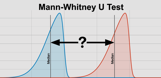
The Mann-Whitney U Test, also called the Wilcoxon Rank Sum Test, is a statistical method used to compare two groups or samples. It is particularly helpful when the data does not meet the assumptions of parametric tests like t-tests. This test helps us understand if two groups likely come from the same population or if they have different distributions regarding a specific variable.
Hypotheses in the Mann-Whitney U Test
- The null hypothesis (H0) suggests that the two populations are equal.
- The alternative hypothesis (H1) states that the two populations are not equal.
Some people mistakenly believe that the Mann-Whitney U Test compares the medians of two groups, while parametric tests compare the means. However, it's important to note that the test statistic for the Mann-Whitney U Test does not directly involve medians. Even if two groups have the same median, they could still be significantly different according to this test.
When to use the Mann-Whitney U Test
Non-parametric tests (sometimes referred to as ‘distribution-free tests’) are used when you assume the data in your populations of interest do not have a Normal distribution. You can think of the Mann Whitney U-test as analogous to the unpaired Student’s t-test, which you would use when assuming your two populations are normally distributed, as defined by their means and standard deviation (the parameters of the distributions).
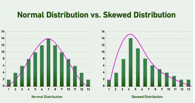
The Mann-Whitney U Test is a common statistical test that is used in many fields including economics, biological sciences, and epidemiology. It is particularly useful when you are assessing the difference between two independent groups with low numbers of individuals in each group (usually less than 30), which are not normally distributed, and where the data are continuous. If you are interested in comparing more than two groups which have skewed data, a Kruskal-Wallis One-Way analysis of variance (ANOVA) should be used.
Mann-Whitney U Test Assumptions
The Mann-Whitney U Test relies on the following key assumptions:
- Continuity of Variable: The variable being analyzed must be continuous, meaning it can take any value within a range (such as age, weight, height, or heart rate). This requirement is because the test involves ranking the data within each group.
- Non-Normal Distribution: The test assumes that the data are not normally distributed (i.e., they are skewed). If the data are normally distributed, the unpaired Student’s t-test would be more appropriate.
- Similar Shape: While the data in both groups do not need to be normally distributed, they should have a similar distribution shape across the groups.
- Independence: The samples must be independent of each other, meaning there is no relationship between the groups. If the samples are paired (e.g., measurements from the same participants), a paired samples t-test should be used instead.
- Sample Size: Each group should have a sufficient number of observations, typically more than 5, to ensure the validity of the test results.
Mann-Whitney U Test Example
Consider a scenario where a study is conducted to evaluate the effectiveness of a new anti-retroviral therapy for HIV. Participants were randomly divided into treated and untreated groups (N=14). The objective is to compare the viral load between the two groups. To analyze this, a Mann-Whitney U Test is commonly used, which can be easily performed using software like SPSS or Stata. Let's delve into the steps involved in performing this test manually.
Data Overview:

Given that the data are both skewed and the sample size is n=7 for each treatment group, a non-parametric test is suitable. Before performing the test, we select a significance level, typically α=0.05.
The initial step involves ranking all values from both treatment groups combined, from the smallest to the largest. This ranking process allows us to calculate the test statistic based on these ranks.
Below is a table displaying the viral load values from the treated and untreated groups, arranged from smallest to largest, along with the summed ranks for each group:
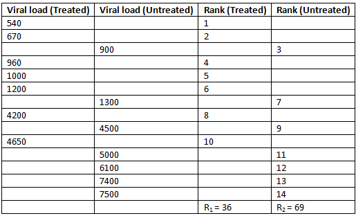
After summing the ranks for each group, the Mann-Whitney U test statistic is selected as the smallest of the two following calculated U values:
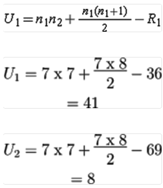
In this analysis, we use 1 to represent the treated group and 2 to represent the untreated group (the choice of group labels is arbitrary). Let n1 and n2 be the number of participants in the treated and untreated groups, respectively, and R1 and R2 be the sums of the ranks for these groups. For this example, U1 = 41 and U2 = 8. We select U = 8 as the test statistic.
Normal Approximation
When sample sizes are large, exact probability distributions might be impractical to use, so we can apply a Normal approximation. According to the central limit theorem, which holds for large sample sizes (typically more than 20 per group), the distribution of U approximates a Normal distribution. By calculating the standard deviation of the rank sums, we can compute a z-statistic and determine a significance value.
Determining the Critical Value:
- To evaluate our test statistic, we compare it to a ‘critical value’ obtained from a reference table, based on our sample sizes (n=7 for each group) and a two-sided significance level (α = 0.05). In this case, the critical value is 8.
Decision Rule:
- Using this critical value, we apply the following rule: reject the null hypothesis (H0) if U ≤ 8. Since our calculated U statistic equals the critical value, we reject H0 and conclude that there is evidence of a significant difference in viral load between the treated and untreated groups.
What is the Kruskal–Wallis test?
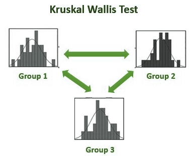
The Kruskal–Wallis test is a method used in statistics to compare two or more groups based on a continuous or discrete variable. It is a non-parametric test, which means it does not make assumptions about the distribution of the data. This test is similar to the one-way analysis of variance (ANOVA). The Kruskal–Wallis test is also known as the one-way ANOVA on ranks or the Kruskal–Wallis one-way ANOVA.
The key points about the Kruskal–Wallis test are as follows:
- The null hypothesis (H0) states that the population medians are equal.
- The alternative hypothesis (H1) suggests that the population medians are not equal, or that the population median of one group differs from the population median of another group.
Kruskal–Wallis test assumptions
Assumptions for the Kruskal–Wallis test are detailed below:
- Data are assumed to be non-Normal or take a skewed distribution. One-way ANOVA should be used when data follow a Normal distribution.
- The variable of interest should have two or more independent groups. The test is most commonly used in the analysis of three or more groups – for analyzing two groups the Mann-Whitney U test should be used instead.
- The data are assumed to take a similar distribution across the groups.
- The data should be randomly selected independent samples, in that the groups should have no relationship to each other.
- Each group sample should have at least 5 observations for a sufficient sample size.
Comparison with Mann–Whitney U test
These assumptions are similar to the Mann–Whitney U test, as the Kruskal–Wallis test is essentially an extension of that test with more than two independent samples. Similar to the Mann-Whitney U Test, the Kruskal–Wallis test is based on ranking the data and calculating a test statistic.
When to use the Kruskal–Wallis test
The Kruskal Wallis test and other non-parametric (or distribution-free) tests are valuable when testing hypotheses without assuming normality of the data. These tests are particularly beneficial when dealing with small datasets because they do not rely on the shape of data distributions.
It's important to understand that non-parametric statistical tests typically yield more conservative results, often presenting a larger p-value compared to parametric tests.
The Kruskal Wallis test is appropriate when the variable of interest is either continuous (capable of taking any number within a range, like age or height) or discrete (representing a specific countable value, such as shoe size, number of hospital visits, or the count of individuals in a household).
Kruskal–Wallis test by hand
A psychologist is intrigued by the link between the sleep patterns of young individuals and their mental well-being. To explore this, they conduct a survey with 15 young people who categorize their average nightly sleep as over 8 hours, 6–8 hours, or less than 6 hours. The psychologist then assesses their mental well-being using a validated score. Below is Table 1 displaying the raw well-being scores collected for each sleep category alongside the median well-being score for each group.
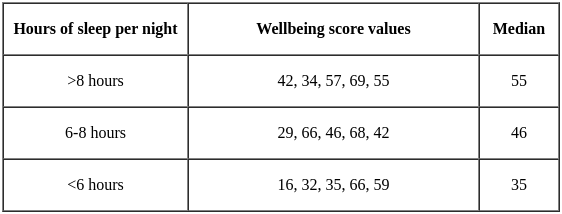
Since we are dealing with a discrete outcome variable, three independent groups, a small sample size, and non-normally distributed groups, the Kruskal–Wallis test is suitable to determine if there are differences in well-being scores across sleep categories.
While common statistical software can easily compute this test, we can manually perform it in five steps.
Step one: Present the null and alternative hypotheses:
The hypotheses are as follows:
- The null hypothesis (H0) states that the median well-being score is the same across sleep groups, or the median differences are zero.
- The alternative hypothesis (H1) suggests that in at least one sleep group, the population median well-being score differs from the population median of another group.
Step two: Sort and assign ranks to the data:
Next, organize all the data in ascending order and assign ranks to the wellbeing scores.

Note: When two scores are the same, the rank given is the average of the ranks that would have been assigned if they were different.
Step three: Add up the ranks for each group:
Calculate the total ranks for each sleeping group by summing up the ranks for each group.
For example:
- T1 (rank total for the <6 hours sleep group): 1 + 3 + 5 + 11 + 12.5 = 32.5
- T2 (rank total for the 6-8 hours sleep group): 2, 6.5, 8, 12.5, 14 = 43
- T3 (rank total for the >8 hours sleep group): 4, 6.5, 9, 10, 15 = 44.5
Step four: Calculate the H statistic:
For the Kruskal-Wallis test, we use a test statistic called the H statistic, computed using the formula:

In the formula, n represents the total number of observations across all groups (e.g., n=15 in this case). Tj denotes the rank total for each group (T1 = 32.5, T T2 = 43, and T), and ni is the number of observations in each group (n1 = 5, n, and n3 = 5). The constant value 12 is part of the formula because it is related to the mean of the sum of squares between ranked groups.
The first part of the formula involves calculating each group’s rank total, squaring it, dividing by the number of observations in that group, and then summing these values. In this formula, j = 1 indicates the starting value of the sum, and c is the final value (in this case, c = 3 because there are 3 groups).
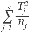

= 396.05 + 369.8 + 211.25 = 977.1
Next, we can plug this value and the total number of observations into the full formula to find H:
= 48.855 - 48.0
= 0.855
This gives us our test statistic of H = 0.855. The degrees of freedom (df) for this test is given by the number of groups minus one, so we have 2 df.
Step five: Obtain and interpret the p-value:
In this final step, we compare the calculated H value to the critical chi-square value and interpret the resulting p-value.
The p-value is obtained from the chi-squared distribution, which is commonly used in nonparametric statistics to represent the distribution of values for a population. In this example, with 2 degrees of freedom and a significance level of 0.05, the p-value is greater than 0.05 because the computed H statistic is significantly smaller than the critical value of 5.991. The exact p-value, calculated using statistical software, is 0.652.
This p-value of 0.652 indicates a high likelihood of observing an H value as extreme as the one we obtained by chance alone. Since this p-value is large, we conclude that there is not enough evidence to reject the null hypothesis, suggesting no significant difference in wellbeing scores among the three sleeping groups.
|
157 videos|236 docs|166 tests
|
FAQs on Mann-Whitney Test (U-Test) & Kruskal-Wallis test (H-test) - Crash Course for UGC NET Commerce
| 1. What is the Mann-Whitney U Test? |  |
| 2. When to use the Mann-Whitney U Test? |  |
| 3. What is the Kruskal-Wallis test? |  |
| 4. When to use the Kruskal-Wallis test? |  |
| 5. What are the Mann-Whitney Test (U-Test) & Kruskal-Wallis test (H-test) used for in UGC NET? |  |


