Unit 2: The Keynesian Theory of Determination of National Income Chapter Notes | Business Economics for CA Foundation PDF Download
Unit Overview
Introduction
In the earlier unit on National Income Accounting, we explored the significance of Gross Domestic Product (GDP) in assessing a country's macroeconomic fundamentals. This unit aims to delve into two key aspects: the factors influencing the level of national income and the process of determining equilibrium aggregate income and output within an economy.
The Great Depression of the 1930s was the most severe economic crisis ever faced by the western world. During this period, classical economists lacked a well-developed theory to explain the persistent problem of unemployment and did not have effective policy recommendations to address it. Although some economists suggested government spending as a means to reduce unemployment, they did not possess a macroeconomic framework to justify their proposals. The field of modern macroeconomics underwent a significant transformation in 1936 with the publication of John Maynard Keynes’s General Theory of Employment, Interest, and Money.
Keynes's General Theory was not merely an academic treatise; it provided clear policy guidance that resonated with the challenges of the Great Depression. In this work, Keynes introduced several foundational concepts of modern macroeconomics, including:
- The relationship between consumption and income, along with the multiplier effect, which explains how shocks to aggregate demand can lead to larger changes in output.
- The concept of Liquidity Preference, referring to the demand for money, which illustrates how monetary policy can influence interest rates and aggregate demand.
- The role of expectations in shaping consumption and investment, emphasizing that changes in expectations are a crucial factor behind shifts in demand and output.
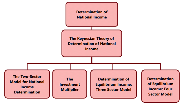
The Keynesian theory of income determination is presented through three models:
(i)The two-sector model, comprising the household and business sectors.
(ii)The three-sector model, which includes the household, business, and government sectors.
(iii) The four-sector model, incorporating the household, business, government, and foreign sectors.
Before diving into the details of income determination in each model, it is essential to grasp the concept of circular flow in an economy, as it underpins the functioning of the entire economic system.
Circular Flow in a Simple Two-Sector Model
Concept of Circular Flow
- The circular flow model illustrates the movement of money within society. In this model: Money flows from producers to workers as wages. Workers then use this money to purchase goods and services from producers, creating a continuous loop. Essentially, the economy functions as an endless circular flow of money.
- This basic model has been expanded by economists to reflect the complexities of modern economies. The additional factors included in the model represent the components of a nation's GDP or national income. This is why the model is also called the circular flow of income model.
- The primary aim of the circular flow model is to understand how money circulates within an economy. It simplifies the economy into two main participants: households and corporations. It also distinguishes between the markets where these participants operate:
(i) Markets for goods and services and
(ii) Markets for factors of production
Role of Households and Corporations
- Households:
- Own all factors of production.
- Sell their factor services to earn incomes, which are then spent on consuming all final goods and services produced by business firms.
- Business Firms:
- Hire factors of production from households.
- Produce and sell goods and services solely to households.
- Do not engage in saving, corporate savings, or retained earnings.
The total income generated in this system, denoted as Y, is received by households and is equal to their disposable personal income, Yd. This relationship is expressed as Y = Yd.
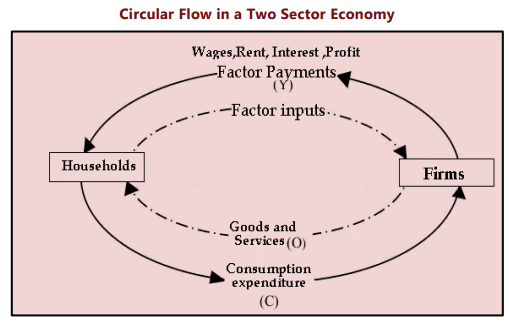
In the circular flow of income and expenditure, as depicted in Figure 1.2.1,
- Real Flows: Represent the flow of actual goods and services.
- Money Flows: Represent payments for these services, such as wages and consumption payments.
In this model: There are no injections or leakages from the system. Household income is entirely spent on goods and services produced by firms.
Factor Payments = Household Income = Household Expenditure = Total Receipts of Firms = Value of Output.
Equilibrium in the Two-Sector Model:
- In the two-sector model, an economy is considered to be in equilibrium when the production plans of firms align with the expenditure plans of households.
Introduction to Keynesian Economics
- The two-sector model is a fundamental representation of Keynesian economics, showcasing the core principles of income determination.
- In this model, the focus is on the ex ante (preliminary) values of various variables, which are crucial for understanding income determination.
Key Concepts in Income Determination
- Before delving into the Keynesian theory of income determination, it is essential to grasp the basic concepts, definitions, and functions that underpin this theory.
Basic Concepts and Functions
Aggregate Demand FunctionAggregate demand (AD) refers to the total planned expenditure in an economy. In a simplified two-sector economy, ex ante aggregate demand for final goods consists of two main components:
- Ex ante aggregate demand for consumer goods (C)
- Ex ante aggregate demand for investment goods (I)
AD = C + I
Consumption Expenditure
- Consumption expenditure is the largest component of GDP in most economies. In a simple model, investment (I) is often considered constant and determined externally in the short run. This leads to the short-run aggregate demand function being primarily influenced by consumption expenditure.
The Consumption Function
- The consumption function illustrates the relationship between aggregate consumption expenditure and aggregate disposable income. It is expressed as:
C = f(Y)
Dissaving at Low Incomes
- When households have low income, their consumption expenditures may exceed their disposable income, leading to dissaving. This can occur through borrowing or using past savings to purchase goods. As disposable income increases, consumers will raise their planned expenditures, but the increase in consumption will be less than the increase in income.
Keynesian Consumption Function
The consumption function proposed by Keynes is given by:
C = a + bY
Key Terms
- C. aggregate consumption expenditure
- Y. total disposable income
- a. constant representing consumption at zero disposable income
- b. marginal propensity to consume (MPC), indicating the increase in consumption per unit increase in disposable income
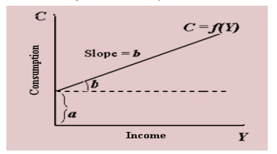
Relationship between Income and Consumption
The average propensity to consume (APC) is a measure that indicates the relationship between total consumption and total income. It is calculated by dividing total consumption by total income. Mathematically, it can be expressed as:
APC = Total Consumption / Total Income = C/Y
The table below illustrates the relationship between income, consumption, saving, average propensity to consume (APC), and marginal propensity to consume (MPC).
Table 1.2.1: Relationship between Income and Consumption

The table illustrates the relationship between income, consumption, and saving. It is important to note that the average propensity to consume (APC) is calculated at various income levels. As income increases, the proportion of income spent on consumption decreases. This raises the question of what happens to the portion of income that is not spent on consumption. Since income can only be spent or saved, the portion not spent must be saved. Therefore, just like consumption, saving is also a function of disposable income, which can be represented as:
S = f(Y)
This relationship between income, consumption, and saving can be further illustrated with the help of a table and a diagram.
In the context of the two-sector model, national income is equivalent to disposable income. The saving function, represented as S = f(Y), shows the relationship between national income and saving. The following table and diagram illustrate this relationship:
Table 1.2.2: Relationship between Income, Consumption, and Saving

The consumption and saving functions can be visualized in the graph. The saving function illustrates the level of saving (S) at each level of disposable income (Y). It is known that consumption at zero income level is positive (equal to a), which also implies dissaving of the same magnitude. According to the definition, national income (Y) is the sum of consumption (C) and saving (S), which can be expressed as:
Y = C + S or S = Y - C
Saving Function and Propensities
- Marginal Propensity to Save (MPS) is the slope of the saving function. It measures how much saving increases with a one-unit increase in disposable income.
- If a one-unit increase in disposable income leads to an increase of ‘b’ units in consumption, then the increase in saving is (1 - b).
- MPS = 1 - b (2.7) (MPS) s = 1-c
- Saving increases as income rises.
- Marginal Propensity to Consume (MPC) is always less than unity and greater than zero, i.e., 0 < b < 1.
- MPC + MPS = 1
- Average Propensity to Save (APS) (2.8)
- APS = Total Saving / Total Income
- Aggregate Supply AS = C + S
ILLUSTRAITION 1
(i)When C = 200 at Y = 1,000
- Total Saving (S) = Y - C = 1,000 - 200 = 800
- Average Propensity to Save (APS) = S / Y = 800 / 1,000 = 0.8
(ii)When S = 450 and Y = 1,200
- Average Propensity to Save (APS) = S / Y = 450 / 1,200 = 0.375
The Two-Sector Model of National Income Determination
In this section, we will explain the two-sector model for determining equilibrium levels of output and income using the aggregate demand and aggregate supply functions. In the Keynesian framework, the equilibrium level of income and output is reached when aggregate demand (C + I) equals aggregate supply (C + S) or output. This can be expressed as: C + I = C + S or I = S (2.9)
Determination of Equilibrium Income: Two Sector Model
In the two-sector model, equilibrium income is determined by the intersection of aggregate demand and aggregate supply. Let's break down the key components:
- Aggregate Demand (AD).This consists of Consumption (C) and Investment (I). It represents the total demand for goods and services in the economy.
- Aggregate Supply (AS).This includes Consumption (C) and Savings (S). It reflects the total output of goods and services in the economy.
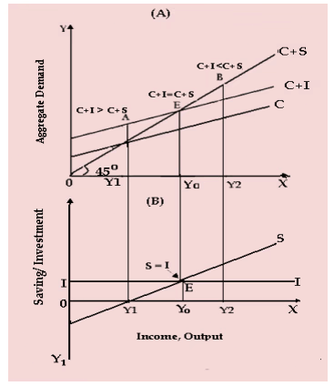
The equilibrium is achieved when I = S, meaning that investment equals savings.
- Aggregate Demand Curve. This curve is linear and positively sloped, indicating that as national income increases, aggregate demand also rises.
- Aggregate Expenditure Line. This line is flatter than the 45-degree line, showing that while consumption increases as income rises, it does so by a lesser amount than the increase in income.
- 45-Degree Line. This line represents points where planned aggregate expenditure equals planned aggregate production. Points on this line indicate that (C + I) = Y or (C + S), mapping out all possible equilibrium income levels.
- Below the 45-Degree Line. At points below this line, planned aggregate expenditure is less than GDP.
- Above the 45-Degree Line. At points above this line, planned aggregate expenditure exceeds GDP.
- Equilibrium Point. The equilibrium is ideally at potential GDP, where planned spending matches production. At point E, aggregate demand equals output, indicating the equilibrium levels of income and output.
- Planned Spending and Production. According to Keynes, aggregate demand (based on households' plans to consume and save) does not always equal aggregate supply (based on producers' plans to produce goods and services). For equilibrium to be established, households' plans must align with producers' plans, where expected value equals realized value.
- Consumers’ consumption plans always align with producers’ production plans, and producers’ investment plans always match households’ saving plans. In other words, there is no reason for consumption plus investment (C + I) and consumption plus savings (C + S) to always be equal.
- The investment function (I) indicates that at equilibrium, planned investment equals savings. Above the income equilibrium level (Y0), savings exceed planned investment, while below this level, planned investment exceeds savings.
- The equality between saving and investment can be directly observed from national income accounting. Since income is either spent or saved, we have Y = C + S.
- In the absence of government and foreign trade, aggregate demand equals consumption plus investment, or Y = C + I. By combining these two equations, we get C + S = C + I, which simplifies to S = I.
- If leakages are greater than injections, national income will fall. Conversely, if injections are greater than leakages, national income will rise.
- National income is in equilibrium only when intended saving equals intended investment. Any deviation from this equilibrium, where planned saving does not equal planned investment, will trigger a readjustment process to bring the economy back to equilibrium.
Equilibrium with Unemployment or Inflation
Deflationary Gap:Deficient Demand refers to a situation where the demand for goods and services in an economy is lower than what is necessary to sustain full employment levels. This leads to a deflationary gap or recessionary gap, indicating that the equilibrium level of aggregate production is falling short of the potential output that could be achieved at full employment.
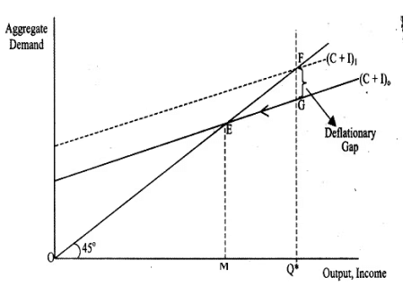
Causes of Deflationary Gap: Deficient Demand can occur due to various factors, such as:
- Decreased consumer confidence, leading to reduced spending.
- Higher interest rates, which discourage borrowing and spending.
- Government austerity measures that cut public spending.
- External factors like global economic downturns affecting demand for exports.
Implications of Deflationary Gap:When there is a deflationary gap, firms experience an unplanned buildup of unsold inventories because the demand for their products is insufficient. In response, they reduce production and lay off workers, leading to a decrease in output and income levels. This process continues until the economy reaches an under-employment equilibrium, where the level of output and employment is below the potential full employment level.
Example:Consider an economy where the full employment level of output is represented by OQ*. For the economy to be at full employment equilibrium, aggregate demand should be at Q*F. However, if aggregate demand falls to Q*G, it indicates deficient demand, creating a deflationary gap FG. Firms will respond by cutting back on production and employment, driving the economy towards a lower equilibrium point E.
(ii) Inflationary Gap
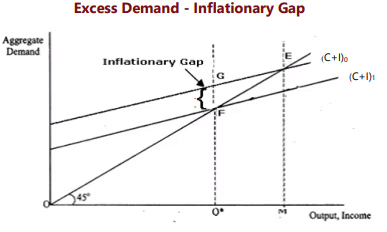
(a) Excess Demand
Excess demand occurs when the aggregate demand for goods and services in an economy exceeds the level that can be sustained at full employment. This situation creates an inflationary gap, which is the difference between actual aggregate demand and the level of demand needed to achieve full employment equilibrium.
(b) Causes of Excess Demand
- Increased consumer spending
- Expansionary fiscal policies, such as tax cuts or increased government spending
- Expansionary monetary policies, like lowering interest rates, which encourage borrowing and spending
- Rapid economic growth in other countries leading to higher demand for exports
(c) Implications of Excess Demand
- When there is excess demand, firms respond to the increased demand by raising prices, leading to demand-pull inflation. This scenario typically occurs during a business-cycle expansion when the economy is growing rapidly.
- The initial effect of excess demand is an increase in the price level, while real output remains constant in the short term. However, over time, nominal output and income rise due to inflation, even though real output and real income may not change immediately.
Example:
- Imagine an economy where the full employment level of output is OQ* and the economy is at full employment equilibrium at point F. If aggregate demand suddenly increases to Q*G, there is excess demand, creating an inflationary gap FG.
- Initially, real output remains the same, but the price level starts to rise, leading to an increase in nominal output and income. This process continues until a new equilibrium is reached at point E, where aggregate demand ME equals output OM. At this new equilibrium, real output, real income, and employment levels remain the same, but nominal output and income have increased due to inflation.
Keynesian Economics and the Great Depression
According to the Keynesian model, during times of abnormally high unemployment and excess capacity, wages and interest rates do not decrease. As a result, output remains below the full employment level unless there is adequate spending in the economy. John Maynard Keynes believed this was the situation during the Great Depression.
Illustration 2: Calculating Marginal Propensity to Consume and Save
Given Data:
- National Income (Y) = 2500
- Autonomous Consumption Expenditure (C̅) = 300
- Investment Expenditure (I) = 100
Equilibrium Condition:
Y = C + I
Substituting the values:
2500 = C + 100
Solving for Consumption (C):
C = 2500 - 100 = 2400
Consumption Function:
C = C̅ + bY
Substituting the values:
2400 = 300 + b(2500)
Rearranging the equation:
2400 - 300 = 2500b
Calculating b:
b = 0.84
Marginal Propensity to Save (MPS):
MPS = 1 - MPC = 1 - 0.84 = 0.16
Illustration 3: Calculation of National Income in Equilibrium
An economy is in equilibrium, and we need to calculate the national income based on the following information:
- Autonomous Consumption (C̅) = 100
- Marginal Propensity to Save (MPS) = 0.2
- Investment Expenditure (I) = 200
Formula: Y = C + I Y = C̅ + MPC (Y) + I where MPC = 1 - MPS
Calculation Steps:
- Step 1: Calculate MPC
- MPC = 1 - MPS = 1 - 0.2 = 0.8
Step 2: Substitute values into the equation
Y = C̅ + MPC (Y) + I
Y = 100 + 0.8Y + 200
Y = 300 + 0.8Y
Step 3: Rearrange the equation
Y - 0.8Y = 300
0.2Y = 300
Step 4: Calculate Y
Y = 300 / 0.2
Y = 1500
Illustration 4: Equilibrium Level of National Income
Given:
- Consumption function: C = 20 + 0.6Y
- Investment function: I = 10 + 0.2Y
To find the equilibrium level of National Income (Y), we use the formula:
Y = C + I
Substituting the values:
Y = 20 + 0.6Y + 10 + 0.2Y
Combining like terms:
Y = 30 + 0.8Y
Rearranging the equation:
Y - 0.8Y = 30
Simplifying:
0.2Y = 30
Therefore:
Y = 30 / 0.2
Y = 150
Illustration 5:
Given: Consumption function: C = 7 + 0.5Y Investment: I = 100
To Find: Equilibrium level of Income (Y), Consumption (C), and Saving (S)
Equilibrium Condition:. = C + I
Substituting the values:. = 7 + 0.5Y + 100
Rearranging the equation:. - 0.5Y = 107
Solving for Y:. = 214
Finding Consumption (C):. = C + I 214 = C + 100 C = 114
Finding Saving (S):. = Y - C S = 214 - 114 S = 100
Summary: Equilibrium Level of Income (Y): 214 Equilibrium Level of Consumption (C): 114 Equilibrium Level of Saving (S): 100
Illustration 6:
Given: Consumption function: C = 250 + 0.80Y Investment: I = 300
To Find: Equilibrium level of Income (Y), Consumption (C), and Saving (S)
Finding Equilibrium Level of Income (Y):. = (1 / (1 - 0.80)) * (250 + 300) Y = (1 / 0.20) * (550) Y = 2750
Finding Consumption (C):. = 250 + 0.80Y C = 250 + 0.80(2750) C = 250 + 2200 C = 2450
Finding Saving (S):. = Y - C S = 2750 - 2450 S = 300
Alternatively:. = -a + (1 - b)Y S = -250 + (1 - 0.80)(2750) S = -250 + (0.20)(2750) S = -250 + 550 S = 300
Summary: Equilibrium Level of Income (Y): 2750 Equilibrium Level of Consumption (C): 2450 Equilibrium Level of Saving (S): 300
Illustration 7: Equilibrium Level of Income and Consumption
Initial Scenario
- Saving function: S = -10 + 0.2Y
- Autonomous investment: I = 50 Crores
- At equilibrium, S = I
- Setting the saving function equal to investment: -10 + 0.2Y = 50
- Solving for Y: 0.2Y = 50 + 10 Y = 300 Crores
- To find consumption (C): C = Y - S
- Calculating S: S = -10 + 0.2 (300) = 50
- Therefore, C = 300 - 50 = 250 Crores
New Scenario with Increased Investment
- If investment increases permanently by 5 Crores, the new investment level becomes 55 Crores.
- Setting the new saving function equal to the increased investment: S = I
- -10 + 0.2Y = 55
- Solving for Y: Y = 325 Crores
- To find the new consumption level (C): C = Y - S
- Calculating S: S = -10 + 0.2 (325) = 65
- Therefore, C = 325 - 65 = 260 Crores
Investment Multiplier
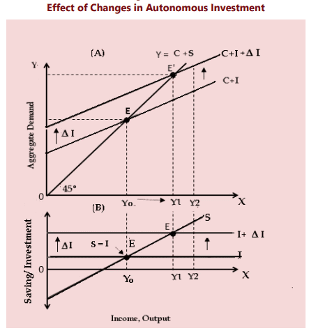
The investment multiplier measures how much the equilibrium level of national income increases in response to a one-unit increase in autonomous investment. It reflects the idea that an increase in investment leads to multiple rounds of increased income and consumption, depending on the marginal propensity to consume (MPC).
Understanding the Investment Multiplier
Calculating the Investment Multiplier
- The investment multiplier (k) is calculated as the ratio of the change in national income (∆Y) to the change in investment (∆I): k = ∆Y / ∆I.
- For example, if an increase in investment of 2000 million leads to an increase in national income of 6000 million, the multiplier is 6000/2000 = 3.
Implications of the Investment Multiplier
- The multiplier indicates how many times the equilibrium national income increases for each unit change in autonomous investment.
- It highlights the significant impact that changes in investment can have on the overall economy, as the effects are not just proportional but multiplicative.
The Multiplier Effect: A Ripple in the Economy
- The multiplier effect can be understood like the ripple effect in water. Imagine a situation where there is an increase in autonomous investment (ΔI) by 500 units. This initial change disrupts the equilibrium and leads to a rise in aggregate demand, which in turn boosts national income. In a two-sector economy, this increase in income is distributed as factor incomes, resulting in a corresponding rise in disposable income.
- As firms experience this heightened demand, they respond by increasing their output. This sets off a chain reaction where the initial rise in investment triggers further increases in consumer demand due to the higher income levels.
- The relationship between the change in equilibrium income and the change in investment is given by the formula: ΔY/ΔI = 1/(1-MPC) = 1/MPS.
- From this, we see that the marginal propensity to consume (MPC) is crucial in determining the value of the multiplier. There is a direct relationship between MPC and the multiplier: the higher the MPC, the greater the multiplier, and vice versa. Conversely, a higher marginal propensity to save (MPS) leads to a lower multiplier.
- The multiplier reaches its maximum value of infinity when MPC is 1, meaning the economy consumes all of its additional income. Essentially, the multiplier value is the inverse of MPS.
- For instance, if MPC is 0.75, the multiplier would be: 1/(1-MPC) = 1/0.25 = 4.
- The multiplier concept is fundamental to Keynesian theory as it explains how changes in investment, driven by shifts in business expectations, lead to variations in both investment and consumption across the economy. It illustrates how shocks in one sector propagate throughout the entire economic system.
- However, the increase in income resulting from initial investment does not continue indefinitely. There comes a point where the process of income propagation slows down and eventually stops. This decline in income is caused by factors known as leakages. Leakages occur when income that could be spent on currently produced consumption goods and services is diverted out of the income stream. When increased income is spent outside the cycle of consumption expenditure, it constitutes a leakage that diminishes the impact of the multiplier. The strength of these leakages is inversely related to the value of the multiplier: the stronger the leakages, the smaller the multiplier.
Leakages can arise from various sources, such as:
- Progressive taxation rates that do not lead to a significant increase in consumption despite higher income.
- High Liquidity Preference and Idle Savings: When there is a high liquidity preference and people are holding onto cash balances, it indicates a fall in the marginal propensity to consume. This scenario reflects a situation where individuals prefer to keep their savings in liquid form rather than spending it.
- Increased Demand for Consumer Goods: In some cases, the increased demand for consumer goods can be met from existing stocks or through imports. This situation arises when there is a sudden surge in demand, but the supply does not immediately adjust to meet this demand.
- Additional Income Spent on Existing Wealth: When additional income is spent on purchasing existing wealth, such as government securities and shares, it indicates a shift in the use of income towards financial assets rather than new consumption.
- Undistributed Profits of Corporations: Undistributed profits of corporations refer to the portion of profits that are retained by the company rather than distributed to shareholders. This can impact the overall consumption and investment dynamics in the economy.
- Increment in Income Used for Debt Payment: Part of the increment in income being used for debt payment indicates a prioritization of reducing liabilities over increasing consumption. This can affect the overall consumption patterns in the economy.
- Full Employment and Additional Investment: In a situation of full employment, any additional investment may lead to inflation rather than an increase in real output. This is because the resources are already fully utilized, and any further investment will push prices up.
- Scarcity of Goods and Services: Even with a high marginal propensity to consume, there can be a scarcity of goods and services. This highlights the structural issues in the economy where increased demand does not lead to an adequate supply response.
- MPC in Underdeveloped Countries: While the marginal propensity to consume is high in underdeveloped countries, the value of the multiplier effect is low. This is due to structural inadequacies where an increase in consumption expenditure does not lead to a corresponding increase in production. For example, a rise in demand for industrial goods due to increased income does not result in a real output increase; instead, prices tend to rise.
- Short-Period Equilibrium in Keynesian Models: Keynesian models are primarily concerned with short-period equilibrium and do not incorporate dynamic elements. When a shock occurs, such as a change in autonomous investment, one equilibrium position can be compared with another through comparative statics. There is no connection between different periods, and the analysis does not account for processes over time.
Illustration 9
In an economy, when investment expenditure increases by ₹ 400 crores and the marginal propensity to consume (MPC) is 0.8, we can calculate the total increase in income and saving as follows:
Given: MPC = 0.8, ∆I = 400 Crores
Step 1: Calculate the Multiplier (K)
Step 2: Calculate the Marginal Propensity to Save (MPS)
Step 3: Calculate the Increase in Income (∆Y)
Step 4: Calculate the Increase in Saving
Summary:
Illustration 10
When investment increases by ₹ 400 crores, it results in a rise in national income by ₹ 1,600 crores. To calculate the marginal propensity to consume (MPC), we can use the following steps:
Given: Increase in investment (∆I) = ₹ 400 crores Increase in national income (∆Y) = ₹ 1,600 crores
Step 1: Calculate the Multiplier (K)
Step 2: Relate the Multiplier to MPC
Step 3: Substitute the Value of K
Step 4: Solve for MPC
Conclusion:
Illustration 11: Impact of Increased Investment on Income and Consumption
When investment in an economy is raised by Rs 600 Crores, with a marginal propensity to consume (MPC) of 0.6, we can calculate the total increase in income and consumption expenditure.
Given.
Calculations.
1. Multiplier (K).
2. Increase in Income (∆Y).
3. Increase in Consumption (∆C).
Results.
Illustration 12: Effect of Increased Investment on Income in a Country
When investment increases by Rs 100 Crores in a country where consumption is defined by the equation C = 10 + 0.6Y (with C representing consumption and Y representing income), we can determine the resulting increase in income.
Given Data.
Calculation of Multiplier (k).
Change in Income (∆Y).
Conclusion.
Equilibrium Income in a Three Sector Model
Y = C + I + G
Since there is no foreign sector involved, Gross Domestic Product (GDP) and national income are considered to be the same. With prices assumed to be fixed, all variables in this model are real variables, and any changes occur in real terms. To better understand these conditions, we can refer to a flowchart that illustrates the circular flow in a three-sector economy. In this model, each variable is treated as a flow variable.
Role of Government Sector
The three-sector, three-market circular flow model with government intervention emphasizes the government’s role. The government sector introduces key flows such as:
- Taxes on households and businesses to finance government purchases.
- Transfer payments to households and subsidies to businesses.
- Government purchases of goods and services from the business sector and factors of production from households.
- Government borrowing in financial markets to cover deficits when taxes are insufficient.
Leakages and Injections
- Unlike the two-sector model, national income does not return directly to firms as demand for output. Households experience leakages through savings and tax payments to the government.
- Savings leak into financial markets, where they are held in the form of financial assets (e.g., currency, bank deposits, bonds, equities). Tax payments flow to the government sector.
- These leakages do not imply a shortfall in total demand. The business sector and government sector also contribute to additional demand through injections.
- Investment is an injection from financial markets to the business sector, where firms typically finance investment goods through borrowing. The amount invested represents a flow of funds lent to the business sector.
In the three-sector Keynesian model, equilibrium national income is determined by the intersection of aggregate demand (AD) and aggregate supply (AS) schedules. Let's break down the key components and concepts involved in this model.
Equilibrium National Income
- Equilibrium national income is achieved when aggregate demand equals aggregate supply, represented by the equation: AD = Y = AS
- This condition ensures that total spending in the economy matches total output, leading to a stable level of income.
Components of Aggregate Demand
- Aggregate Demand (AD) is the total demand for goods and services in the economy, given by the sum of consumption (C), investment (I), and government spending (G): AD = C + I + G
- Consumption (C) is the total spending by households on goods and services.
- Investment (I) includes spending by businesses on capital goods and residential construction.
- Government Spending (G) refers to expenditures by the government on goods and services.
Components of Aggregate Supply
- Aggregate Supply (AS) represents the total supply of goods and services in the economy, which is equal to the sum of consumption (C), savings (S), and taxes (T): AS = C + S + T
- Savings (S) is the portion of income that is not consumed.
- Taxes (T) are mandatory contributions levied by the government on individuals and businesses.
Equilibrium Condition
- The equilibrium level of income is reached when the aggregate demand schedule (C + I + G) intersects the 45-degree line, indicating that total spending equals total output.
- At this point, it is also true that the aggregate supply schedule (S + T) intersects the autonomous expenditure components (I + G), maintaining the balance between supply and demand.
Explanation of Non-Equilibrium Points
- Below Equilibrium (Y Y ) : At income levels below Y Y , consumption is lower than the potential, leading to excess demand. The aggregate demand exceeds income, resulting in unintended inventory shortfalls and a tendency for output to rise.
- At Equilibrium (Y Y ) : At the equilibrium point Y Y , aggregate demand equals aggregate supply, and there are no unintended inventory changes. This balance reflects the stability of output and employment levels.
- Above Equilibrium (Y Y ) : At income levels above Y Y , output exceeds demand, causing excess inventory accumulation. Businesses respond by reducing production, leading to a decline in employment and output until equilibrium is restored.
- In the Keynesian model, it is the change in total spending that triggers adjustments in output and employment to restore equilibrium. Price changes do not play a significant role in this adjustment process.
- When there is an increase in total spending, it leads to higher demand, prompting businesses to increase production and hire more workers, thereby raising output and employment levels. Conversely, a decrease in total spending results in lower demand, causing businesses to reduce production and employment, bringing the economy back to equilibrium.
The Role of the Government Sector in Income Determination
The government plays a significant role in influencing the level of income through various means such as taxes, transfer payments, government purchases, and government borrowing. While a detailed discussion on government fiscal policy is beyond the scope of this unit, we will focus on a few key variables.
(i) Income Determination with Lump Sum Tax
- Lump Sum Tax: We assume the government imposes a lump sum tax, which is a tax that does not depend on income.
- Balanced Budget: The government has a balanced budget, meaning government spending (G) equals tax revenue (T).
- No Transfer Payments: There are no transfer payments in this scenario.
- Consumption Function: The consumption function is given by C = a + b Yd, where Yd is disposable income (Y - T), T is the lump sum tax, and Y is national income.

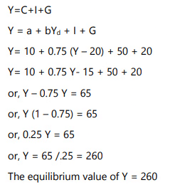
Illustration 13: Finding Equilibrium National Income and Multiplier
In this illustration, we have data from a simple economy where:
The equations given are:
(a) Finding the Equilibrium Level of National Income
To find the equilibrium level of national income (Y), we substitute the values of C, I, and G into the national income identity:
(b) Size of the Multiplier
The size of the multiplier (k) can be calculated using the formula:
k = 1 / (1 - MPC)
Where MPC is the marginal propensity to consume. In this case, MPC = b = 0.75.
k = 1 / (1 - 0.75) = 1 / 0.25 = 4
(ii) Income Determination with Lump Sum Tax and Transfer Payments
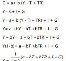
When considering lump sum tax (T) and autonomous transfer payments (TR), the disposable income is given by:
Yd = Y - T + TR
Illustration 14: Finding Equilibrium Level of Income
Given: Consumption function. C = 100 + 0.75Yd Investment. I = 200 Government Spending. G = 100 Taxes. T = 100 Transfer Payments. TR = 50
To find the equilibrium level of income (Y)
Step 1: Write the income identity
Y = C + I + G
Step 2: Substitute the consumption function
Y = 100 + 0.75Yd + 200 + 100
Step 3: Substitute for disposable income (Yd)
Yd = Y - T + TR = Y - 100 + 50 = Y - 50
Step 4: Substitute Yd into the equation
Y = 100 + 0.75(Y - 50) + 200 + 100
Step 5: Simplify the equation
Y = 100 + 0.75Y - 37.5 + 200 + 100
Y = 100 + 0.75Y + 262.5
Step 6: Combine like terms
Y - 0.75Y = 462.5
0.25Y = 462.5
Step 7: Solve for Y
Y = 462.5 / 0.25 Y = 1850
Alternative Method: Using the formula
Y = 1 / (1-b) (a - bT + bTR + I + G)
Where:
Step 1: Calculate (1-b)
1 - b = 1 - 0.75 = 0.25
Step 2: Substitute values into the formula
Y = 1 / (0.25) (100 - 0.75(100) + 0.75(50) + 200 + 100)
Y = 4 (100 - 75 + 37.5 + 200 + 100)
Y = 4 (362.5)
Y = 1450
Income Determination with Tax as a Function of Income
In the previous analyses, we explored the impact of a balanced budget with an autonomous lump sum tax. However, in reality, the tax system comprises both lump sum taxes and proportional taxes. The tax function can be defined as:
Tax Function: T = T̅ + tY
- T̅- Autonomous constant tax
- t- Income tax rate
- T- Total tax
Disposable Income (Yd): Yd = Y - T = Y - T̅ - tY
Consumption Function: C = a + b(Y - T̅ - tY)
Equilibrium Level of National Income:
Y = C + I + G
Y = a + bYd + I + G
Y = a + b(Y - T̅ - tY) + I + G
Y = a + bY - bT̅ - btY + I + G
Y - bY + btY = a - bT̅ + I + G
Y (1 - b + bt) = a - bT̅ + I + G
Y = 1 / (1 - b(1 - t)) (a - bT̅ + I + G)
Where: 1 / (1 - b(1 - t)) represents the tax multiplier.
Illustration 15
Given Data for a Closed Economy:
(a) To find the equilibrium income (Y):
1. Start with the equilibrium condition: Y = C + I + G
2. Substitute the values: Y = 75 + 0.5(Y - 25 - 0.1Y) + 80 + 100
3. Simplify the equation:
Y(1 - 0.5 + 0.05) = 75 - 12.5 + 80 + 100
4. Solve for Y: Y ≈ 440.91
(b) To find the value of the multiplier:
1. Use the formula: Multiplier = 1 / [1 - b(1 - t)]
2. Substitute the values: Multiplier = 1 / [1 - 0.5(1 - 0.1)] ≈ 1.82
Determination of Equilibrium Income: Four Sector Model
The four sector model considers the interactions between the household sector, business sector, government sector, and foreign sector. In this model, the circular flow of income includes exports, imports, and net capital inflow, which is the difference between capital outflow and capital inflow.
Circular Flow in a Four Sector Economy
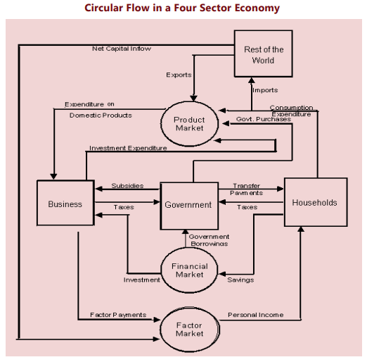
In equilibrium, national income (Y) is equal to the sum of consumption (C), investment (I), government spending (G), and net exports (X-M), as shown in the equation:
Y = C + I + G + (X-M)
Exports are considered injections into national income, as they represent foreign demand for domestic goods. On the other hand, imports are leakages from national income, as they represent goods produced abroad. The demand for imports is influenced by income and is expressed through the import function:
- M = M̅ + mY
Where:
- M̅ is the autonomous component of imports,
- m is the marginal propensity to import, and
- Y is national income.
The marginal propensity to import (m) is the increase in import demand per unit increase in GDP and is assumed to be constant.
Net exports (X-M) represent the foreign sector's contribution to aggregate expenditures and are calculated by subtracting imports from exports. While export demand is determined by foreign income and is therefore autonomous, the demand for imports is influenced by both the autonomous component and income.
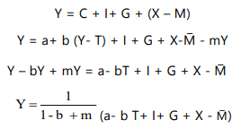
The equilibrium level of national income is achieved when aggregate demand equals aggregate supply, as represented by the equation:

The equilibrium level of National Income can now be expressed by –
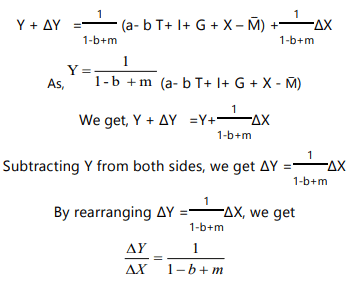
The economy being in equilibrium, suppose export of country increases by ∆ X autonomously, all other factors remaining constant. By incorporating the increase in exports by ∆ X, the equilibrium equation of the country can be expressed as

or
Or alternatively written as

The term  is known as foreign trade multiplier whose value is determined by marginal propensity to consume (b) and marginal propensity to import (m)
If in the model proportional income tax and government transfer payments are incorporated, then only the denominator of multiplier will change.
If income tax is of form T = T ̅ + t Y where T ̅ is constant lump-sum, t is the proportion of income tax and TR > 0 and autonomous, then the four sector model can be expressed as: –

The equilibrium level of National Income can now be expressed as:

Effects on Income When Imports are Greater than Exports
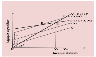
- In the previous section, we learned that equilibrium income is determined by multiplying two factors: the level of autonomous investment expenditure and the investment multiplier.
- In a four-sector model, the autonomous expenditure multiplier accounts for foreign transactions. It is calculated using the formula where 'm' represents the propensity to import, which is greater than zero 1/(1−𝑏+𝑚) .
- In a closed economy, the multiplier is (1−𝑏).
- A higher value of 'm' leads to a lower autonomous expenditure multiplier. This means that in a more open economy with higher imports, the response of income to aggregate demand shocks, such as changes in government spending or investment demand, becomes smaller.
- When 'm' is high, a larger proportion of the induced effect is directed towards foreign consumer goods instead of domestic ones.
- The increase in imports per unit of income represents an additional leakage from the circular flow of domestic income at each round of the multiplier process, reducing the value of the autonomous expenditure multiplier.
In this illustration, we are given a consumption function along with values for taxes, investment, government spending, exports, and imports. We are required to find the equilibrium level of income, net exports, and how net exports change with an increase in exports.
Consumption Function
The consumption function is given by:
C = 40 + 0.8Yd
Where:
Disposable income (Yd) is calculated as:
Yd = Y - T
Given that T = 0.1Y (taxes), we can rewrite the consumption function as:
C = 40 + 0.8(Y - 0.1Y)
C = 40 + 0.8(0.9Y)
Equilibrium Condition
At equilibrium, total output (Y) is equal to total spending, which includes consumption (C), investment (I), government spending (G), and net exports (X - M).
Y = C + I + G + (X - M)
Substituting the given values:
Y = 40 + 0.8(0.9Y) + 60 + 40 + (58 - 0.05Y)
Y = 40 + 0.72Y + 60 + 40 + 58 - 0.05Y
Solving for Y
Combine like terms:
Y - 0.72Y + 0.05Y = 198
Y(1 - 0.72 + 0.05) = 198
Y(0.33) = 198
Y = 198 / 0.33 = 600 Crores
Net Exports
Net exports are calculated as:
Net Exports = X - M
Substituting the values:
Net Exports = 58 - 0.05Y
= 58 - 0.05(600)
= 58 - 30
= 28 Crores
Impact of Increase in Exports
If exports were to increase by 6.25, the new value for exports would be:
New Exports = 64.25
Recalculate Y:
Y = 40 + 0.8(Y - 0.1Y) + 60 + 40 + (64.25 - 0.05Y)
Y(1 - 0.72 + 0.05) = 204.5
Y(0.33) = 204.5
Y = 204.5 / 0.33 = 619.697 Crores
Calculate new imports:
M = 0.05 × 619.697 = 30.98 Crores
Calculate new net exports:
Net Exports = 64.25 - 30.98 = 33.27 Crores
Conclusion
There is a surplus in the balance of trade as net exports are positive.
|
86 videos|255 docs|58 tests
|
FAQs on Unit 2: The Keynesian Theory of Determination of National Income Chapter Notes - Business Economics for CA Foundation
| 1. What is the circular flow model in a simple two-sector economy? |  |
| 2. How does equilibrium with unemployment differ from equilibrium with inflation? |  |
| 3. What is the investment multiplier, and how does it function in the economy? |  |
| 4. How is equilibrium income determined in a three-sector model involving households, firms, and the government? |  |
| 5. What role does the government sector play in income determination in the four-sector model? |  |


