ANOVA, Correlation and Data Reduction

ANOVA

• Prof. R. A. Fisher first used the term variance and developed a detailed theory of ANOVA.
• He explained how ANOVA is useful for practical research applications.
• ANOVA is a procedure to test whether different groups of data are homogeneous.
• It partitions the total variation in a data set into two parts: variation due to chance and variation due to specific causes.
• ANOVA splits variance into components for analytical purposes.
• It analyses the variance of a response by assigning components to different sources of variation.
• Using ANOVA, one can study any number of factors believed to affect the dependent variable.

Types of ANOVA

These are as follows:

One-Way ANOVA

• One-way ANOVA tests differences among two or more independent groups.
• It is typically applied when comparing three or more groups, because two-group cases can be handled by Student's t-test.
• When only two means are compared, the t-test and the F-test are equivalent with F = t².
• For example, a researcher might compare students' attitude towards school across school types: SSC, CBSE and ICSE.
• Here the dependent variable is attitude towards the school and the groups are SSC, CBSE and ICSE schools.
• One-way ANOVA tests whether students' attitudes differ among these three groups.
• One-way repeated measures ANOVA is used when the same subjects receive repeated measurements.
• That is, the same subjects are measured under each treatment.
• This design can be affected by carry-over effects.
• It is commonly used in experiments comparing three or more related measurements, for example pre-test and post-test scores.

Two-Way ANOVA

• Two-way ANOVA studies the effects of two independent or treatment variables.
• It is also called factorial ANOVA.
• The most common factorial design is 2 × 2, meaning two independent variables each with two levels.
• Two-way ANOVA can have higher levels such as 3 × 3 or higher-order designs like 2 × 2 × 2.
• Manual calculations for many factors are lengthy, so higher-order analyses became common after data analysis software emerged.
• For example, a researcher might compare students' attitude by school type (SSC, CBSE, ICSE) and gender.
• Here the dependent variable is attitude towards the school and the independent variables are school type (three levels) and gender (two levels).
• This would be a 3 × 2 two-way ANOVA, testing attitude differences by school type and gender.

MANOVA

• When samples receive repeated measures, such as pre-test and post-test, a factorial mixed design can be used: Multivariate Analysis of Variance (MANOVA).
• In MANOVA one factor may be a between-subjects variable and the other a within-subjects variable.
• This is a type of mixed-effects model.
• MANOVA is used when there is more than one dependent variable.

ANCOVA

• When comparing two groups on a dependent variable, initial differences on another variable (for example SES or pre-test scores) should be removed.

Assumptions of Using ANOVA

• Independence of cases.
• Normality of the distribution in each group.
• Equality or homogeneity of variances (homoscedasticity); group variances should be similar.
• Levene's test is commonly used to check homogeneity of variances.
• The Kolmogorov-Smirnov or Shapiro-Wilk tests may be used to test normality.
• Lindman argues that the F-test is unreliable when distributions deviate from normality.
• Ferguson and Takane claim the F-test is robust to such deviations.
• The Kruskal-Wallis test is a non-parametric alternative that does not assume normality.

Chi-Square (Equal Probability and Normal Probability Hypothesis)

• A chi-square test (also chi-squared or χ² test) is any statistical test whose test statistic follows a chi-square distribution when the null hypothesis holds.
• More generally, the test statistic's distribution can be made to approximate a chi-square distribution as sample size increases.
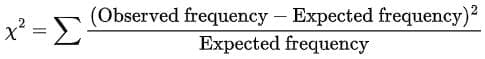
• Chi-square tests are commonly used to compare observed data with expected frequencies under a specified hypothesis.
• For example, if a researcher expects parents' attitudes towards sex education to follow a particular distribution, the chi-square test checks whether observed counts fit those expectations.
• The null hypothesis states there is no significant difference between observed and expected results.
• If expected frequencies are assumed equal across cells, the test is the equal distribution hypothesis.
• If expected frequencies follow a normal distribution, it is the normal distribution hypothesis.
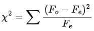
• The chi-square (χ²) test measures agreement between two sets of frequency counts.
• These must be categorical counts, not percentages or ratios.

Thus,

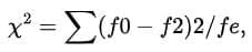
• fo denotes observed frequency and fe denotes expected frequency.
• Expected values may need scaling to match observed totals.
• Total counts for observed and expected values should be equal.
• In a contingency table, expected frequency can be estimated as fe = (row total × column total) / N.
• Here N is the grand total of all cells.
• The calculated chi-square is compared with table values to assess significance.

In a table, the degrees of freedom are computed as follows:

• df = (R - 1) × (C - 1)
• Where R = number of rows and C = number of columns.
• Chi-square indicates whether a significant association exists between variables but does not measure the strength or importance of that association.
• χ² is the most used non-parametric test for comparing sample distributions with theoretical or established distributions.
• It is useful when the population distribution cannot be assumed to be normal.
• Advantages of chi-square tests include being distribution-free, easy to compute, and applicable when parametric tests are not suitable.
• The χ² test was first used by Karl Pearson in 1890.
• Chi-square can also compare two or more actual samples.

Steps in the Calculation of χ

²

• First compute expected frequencies (E) using the formula shown in the image below.

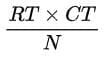
• RT = row total for the row containing the cell.
• CT = column total for the column containing the cell.
• Compute O - E for each cell.
• Divide (O - E)² by E for each cell and then sum across all cells.
• χ² ranges from zero to infinity; zero indicates perfect agreement between observed and expected counts.
• Larger discrepancies between O and E produce larger χ² values.

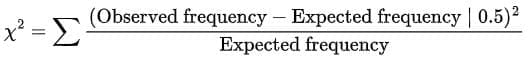
Basic Computational Equation

(Observed frequency - Expected frequency)²

• Therefore, accept the null hypothesis.
• When there is one degree of freedom, Yates' correction for continuity should be applied.
• This correction subtracts 0.5 from the absolute value of each cell's numerator contribution before squaring.
• The adjusted chi-square formula with Yates' correction is shown in the image below.

• In χ², the sum of (O - E) over all cells equals zero: ∑(O - E) = N - N = 0.
• This provides a check on chi-square computations.
• χ² depends only on observed and expected frequencies and the degrees of freedom.
• The χ² distribution approximates the multinomial distribution and applies to discrete frequency counts.

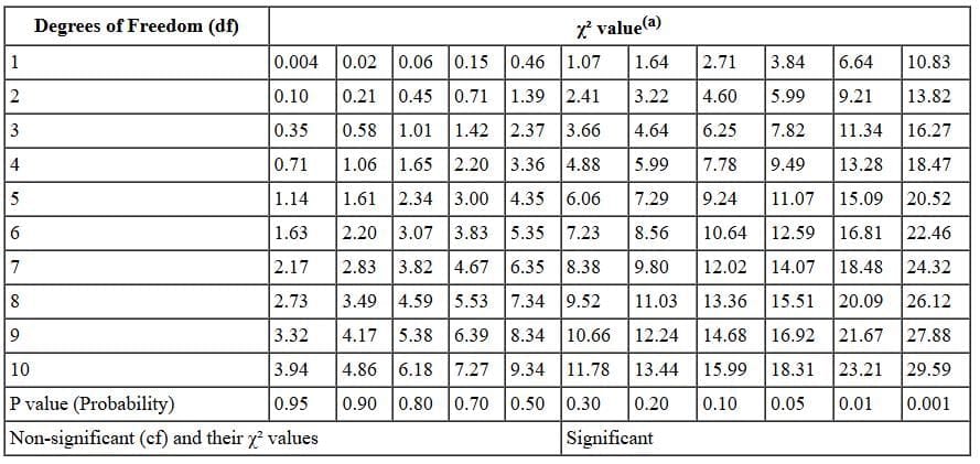
Level of Significance

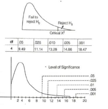
• The calculated χ² is compared with the table value for a given degree of freedom at a chosen significance level.
• Usually a 5% level of significance is selected.
• If χ² > table value, the difference between theory and observation is considered significant.
• χ² is a random variable that varies by sample and is always non-negative.
• χ² is a statistic derived from data, not a population parameter.

Above table represents a graph for degrees of freedom equal to 4 at different significance levels.

Uses of χ

²

 Test

• χ² test as a test of independence: it checks whether two or more attributes are associated.
• To test association, the null hypothesis assumes no relationship between the attributes.
• If χ² is less than the table value at the chosen significance level, we do not reject the null hypothesis; the attributes appear unrelated.
• If χ² > table value, we reject the null hypothesis and infer the attributes are related.
• χ² test as a goodness-of-fit test: it shows how well a theoretical distribution fits observed data.
• It compares an ideal frequency curve with observed facts to assess fit.
• χ² test as a test of homogeneity: it determines whether two or more independent samples come from the same population.

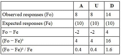
Example: If a fair coin is flipped 20 times, we expect 10 heads and 10 tails, though sampling error can produce variations such as 12 heads and 8 tails.

If the experiment yielded 12 heads and 8 tails, we enter expected (10, 10) and observed (12, 8) frequencies into a table.

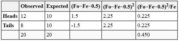
• With Yates' correction, subtract 0.5 from the absolute difference between observed and expected in each category before squaring.
• Divide the squared result by the expected frequency and sum across categories to compute χ².
• How does a calculated χ² of 0.450 inform us about the coin flip result 12 vs 8?
• The chi-square sampling distribution shape depends on degrees of freedom.
• For a one-way χ² test, degrees of freedom equal r - 1, where r is the number of levels.
• Here r = 2, so df = 1.
• From tables, χ² ≥ 3.84 is needed for significance at the 0.05 level with 1 df.
• Our χ² = 0.450 is less than 3.84, so the deviation could be due to sampling error and is not significant at the 0.05 level.

Different Levels of Significance

Correlation

• Correlation is a statistical measure of the relationship between two variables.
• It quantifies both the strength and direction of that relationship.
• Each subject must have two measures to compute correlation.
• If two quantities change together, they are said to be correlated.
• The degree of correlation indicates how strongly the two variables are related.
• This degree is summarised by the correlation coefficient.
• Two independent variables are not correlated because they lack a meaningful relationship to interpret.
• The correlation coefficient ranges from -1 to +1; -1 is perfect negative, +1 is perfect positive, and 0 means no correlation.
• Correlation analysis can determine whether a relationship exists, its direction (positive or negative), and whether it is statistically significant.
• Correlation analysis may also be used in attempts to establish cause-and-effect, though correlation alone does not prove causation.

Types of Correlation

There are different types of correlation, as follows:

• Positive correlation occurs when both variables move in the same direction; for example, higher intelligence associated with higher adjustability.
• This is denoted by a plus (+) sign.
• Negative correlation occurs when the variables move in opposite directions; one increases while the other decreases.
• This is denoted by a minus (-) sign.
• A zero coefficient indicates no relationship between the variables.

Simple, Partial and Multiple Correlation

• These distinctions depend on the number of variables studied.
• Simple correlation involves two variables.
• Partial correlation considers more than two variables but examines the relationship between two variables while holding others constant.
• Multiple correlation studies the relationship among three or more variables simultaneously.

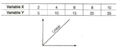
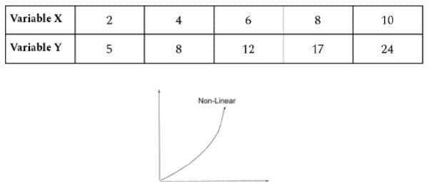
Linear and Non-Linear Correlation

• Linear correlation means the variables vary in a constant ratio and the relationship remains at a constant rate.

• If percentage changes in X and Y are not constant and fluctuate, the relationship is non-linear or curvilinear.

Methods of Studying Correlation

These are:

• Scatter diagram
• Correlation graph
• Product-moment coefficient of correlation
• Rank-difference correlation method
• Coefficient of concurrent deviation
• Method of least squares

Uses of Correlation

• To evaluate reliability and validity of psychological tests and inventories.
• In factor analysis techniques.
• To make predictions.
• In path analysis techniques.

Two Methods of Correlation

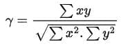
Product-Moment Method of Coefficient

• Pearson's coefficient is commonly denoted by r.
• It is used when the relationship between two variables is linear.
• It applies when data for X and Y are at interval or ratio level and the distribution is linear.
• The term product-moment refers to the mean of the product of mean-adjusted random variables.
• It measures the strength and direction of the linear relationship and equals the sample covariance divided by the product of the standard deviations.

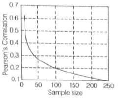
A graph shows the minimum Pearson correlation that is significantly different from zero at the 0.05 level for given sample sizes.

• There are two calculation methods for Pearson's coefficient:
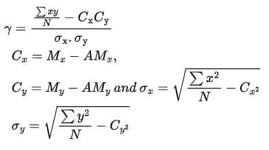
• Long method (actual mean method)
• Short method (assumed mean method)

For the actual mean method:

• Care points:
• If ∑xy is large relative to ∑x² and ∑y², the correlation will be high, and vice versa.
• If ∑xy is negative, the correlation coefficient will be negative.
• The degree of y indicates the degree of variation between the two series.

Rank-Order Coefficient of Correlation

• Used when data are ranks rather than scores.
• It applies when the relationship is not linear and product-moment methods are inappropriate.
• In such cases, the rank-order method uses Spearman's rho (ρ) to measure association.

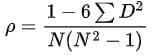
• Where D = difference in ranks for a pair and N = number of pairs.
• ρ = coefficient of correlation by rank-order method.

Significance of Correlation Coefficient

• From 0.00 to 0.20 denotes negligible relationship.
• From 0.20 to 0.40 denotes slight correlation.
• From 0.40 to 0.70 denotes substantial or marked relationship.
• From 0.70 to 1.00 denotes high to very high relationship.

Z-Test

• A Z-test is a type of hypothesis test that helps assess whether test results are likely to be true or repeatable.
• A hypothesis test determines whether findings are probably true or probably not true.
• A Z-test is used when data are approximately normally distributed.

When to Use a Z-Test

• Use a Z-test when your sample size is greater than 30; otherwise use a t-test.
• Data points should be independent of each other.
• Data should be normally distributed, though large samples reduce this concern.
• Samples should be randomly drawn so each item has equal selection chance.
• Prefer equal sample sizes where possible.

One-Sample Z-Test Example

• An investor tests whether a stock's average daily return exceeds 1%.
• A random sample of 50 returns has a mean of 2% and an assumed population standard deviation of 2.50%.
• The null hypothesis states the mean equals 1% and the alternative states the mean is greater than 1%.
• Assume α = 0.05 with a two-tailed test, so critical z values are ±1.96.
• Z is computed as (observed mean - test mean) divided by (standard deviation / √n).
• Here z = (0.02 - 0.01) / (0.025 / √50) ≈ 2.83.
• Since 2.83 > 1.96, the investor rejects the null hypothesis and concludes the mean return is greater than 1%.

Qualitative Data Analysis

• Qualitative data are verbal or symbolic materials describing behaviours, people, situations and events.
• Analyzing qualitative data means studying organised material to discover underlying facts.
• Researchers examine the data from many angles to explore new facts or reinterpret known ones.

The types of qualitative data analysis are:

Data Reduction

• Data reduction involves selecting, focusing, simplifying, abstracting and transforming data from field notes or transcriptions.
• Raw data must be organised and meaningfully condensed to become manageable.
• Reduction transforms data to make them intelligible for the research questions.
• Researchers use the principle of selectivity to choose which data to describe.
• Data reduction typically combines deductive and inductive analysis.
• Coding is done by discussion topics, observation checklists or semi-structured interview guides.

Classification

• Classification groups items by shared attributes to create categories or typologies.
• Historically, science emphasised classification systems; examples include botanical classifications and the periodic table.
• Analysts look for recurring patterns in categorized data and form classification systems accordingly.
• Categories are judged by internal homogeneity and external heterogeneity.
• A large number of unassignable or overlapping items suggests faults in the category system.
• Analysts iteratively refine categories by checking data placement and category meaningfulness.
• Priorities among classification schemes are set by salience, credibility, uniqueness, feasibility and materiality.
• Completeness is tested by internal and external checks to ensure categories are consistent and form a coherent whole.
• Category building involves both technical and creative work; no infallible procedure exists.
• In summary: identify and develop categories, judge them for homogeneity and heterogeneity, assign data, recheck and prioritise categories, test for completeness, and label categories clearly.

Analytical Induction

• Analytical induction builds explanations by creating and testing causal links within cases and extending these to other cases.
• It is a research logic used to collect data, develop analysis and structure research findings.
• Its goal is causal explanation and it originated from symbolic interaction theory.
• It searches for broad categories and then develops sub-categories; definitions are refined as analysis progresses.
• If similarities are not found, data or definitions are re-evaluated or categories narrowed.
• Definitions are treated as hypotheses to be tested and revised using inductive reasoning.
• Katz defined analytic induction as a logic to collect data, develop analysis and present findings.
• AI calls for progressive redefinition of the phenomenon and explanatory factors to maintain a universal relationship.
• Initial cases suggest provisional explanations which are revised as contradictory cases appear.
• Cressey outlined analytical induction steps as:
• Define the phenomenon tentatively.
• Develop a hypothesis about it.
• Examine a single instance to test the hypothesis.
• If the hypothesis fails, redefine the phenomenon or revise the hypothesis to include the instance examined.
• Examine additional cases; if the hypothesis continues to hold, confidence increases.
• Each negative case requires reformulation until no exceptions remain.

Constant Comparison

• Constant comparison analyses qualitative data to develop theory and is central to grounded theory methods.
• It involves comparing newly coded passages with previously coded passages to ensure consistent coding.
• This helps to identify passages that may be better coded differently or that reveal new dimensions.
• Comparisons can extend across cases or even to external examples to refine codes.
• New data are constantly compared with existing data to refine theoretical categories and guide the research.

Strauss and Corbin (1990) recommend these components for constant comparison:

• Word repetitions - look for frequently used words and repeats that indicate emotions.
• Indigenous categories - use terms respondents use with special meaning (in vivo codes).
• Key words in context - examine the range of a term's uses in phrases and sentences.
• Compare and contrast - ask what a passage is about and how it differs from adjacent statements.
• Social science queries - introduce explanations to account for conditions, actions and consequences.
• Searching for missing information - look for expected but absent phenomena.
• Metaphors and analogies - metaphors may reveal central beliefs and feelings.
• Transitions - note discursive elements like turn-taking and narrative structures.
• Paging - mark and scan text using highlights and marginal lines to identify patterns.
• Cutting and sorting - collect all similarly coded transcript excerpts together to review and analyse them as a set.

Triangulation

• Triangulation uses more than one method to collect data on the same topic.
• It validates data by cross-verification from multiple sources.
• Triangulation tests consistency across instruments and helps assess multiple causes influencing results.
• It deepens and broadens understanding rather than only providing validation.
• Triangulation is used in both qualitative and quantitative research.

The term originated in surveying and navigation and was adopted in social science as a metaphor for multiple operationalisation.

• Campbell and Fiske first applied the term triangulation to research to describe multiple data collection strategies measuring a single concept (data triangulation).
• The purpose of triangulation is to relate different kinds of data to enhance validity and understanding.

Types of Triangulation

They include:

• Data triangulation (time, space and person)
• Method triangulation (design and data collection)
• Investigator triangulation
• Theory triangulation
• Multiple triangulation, which combines two or more triangulation techniques

• Denzin (1989) described three types of data triangulation:
• Time triangulation - collecting data about a phenomenon at different times; note this differs from longitudinal studies meant to document change.
• Space triangulation - collecting data at more than one site to distinguish time- or space-specific characteristics.
• Person triangulation - collecting data from multiple levels of persons (individuals, groups or collectives); Denzin describes aggregate, interactive and collective levels.

Smith lists seven levels of person triangulation:

• (i) Individual level
• (ii) Group analysis - interaction patterns among individuals and groups
• (iii) Organisational units of analysis - units that have qualities beyond the individuals
• (iv) Institutional analysis - relationships across legal, political, economic and familial institutions
• (v) Ecological analysis - spatial explanations
• (vi) Cultural analysis - norms, values, practices and ideologies of a culture
• (vii) Societal analysis - broad factors like urbanisation, industrialisation, education and wealth

• Methods triangulation can occur at the design level or the data collection level.
• Design-level triangulation (between-method) combines quantitative and qualitative methods in the study design, either simultaneously or sequentially.
• Data-collection triangulation (within-method) uses two different techniques within the same research tradition to gain a fuller understanding of the phenomenon.
• Method triangulation can be time-consuming and expensive but often yields richer insights.

• Investigator triangulation involves multiple researchers with diverse backgrounds collaborating on the same study.
• Each investigator should have a distinct, complementary role.

• Theory triangulation uses different theoretical perspectives to interpret the same data.
• This strategy enhances research quality and helps reveal multiple theoretical explanations.
• Researchers cycle between data generation and analysis to test emerging theories until conclusions are reached.

• Denzin recommends combining multiple methods, data sources and investigators to identify and validate issues.
• Multiple methods reveal different aspects of reality and together increase trustworthiness and comprehensiveness.
• Guba argues triangulation enhances credibility, dependability and confirmability in qualitative research.