Unemployment - Phillips Curve Analysis


Introduction
The Phillips curve is an economic model that relates the rate of inflation to the rate of unemployment. It is named after A. W. (Bill) Phillips, who in 1958 documented a negative relationship between the rate of wage inflation and the unemployment rate in the United Kingdom. The observation was subsequently developed into an explicit inflation‐unemployment relation by economists such as Paul Samuelson and Robert Solow.
Later theoretical work by Milton Friedman and Edmund Phelps introduced expectations into the analysis and argued that any trade‐off between inflation and unemployment is, at best, temporary. The Phillips curve therefore has both a short‐run interpretation, where a downward-sloping trade‐off may appear, and a long‐run interpretation, where this trade‐off disappears.
During the 1950s and 1960s evidence seemed to support a policy choice between lower unemployment and higher inflation. However, the experience of the 1970s - when many economies experienced simultaneous high inflation and high unemployment (known as stagflation) - showed limitations of the simple Phillips curve and prompted deeper analysis of expectations and supply shocks. Despite its limitations, the Phillips curve framework remains important for understanding interactions between inflation, unemployment and expectations in macroeconomic policy.
Origins of the Phillips Curve
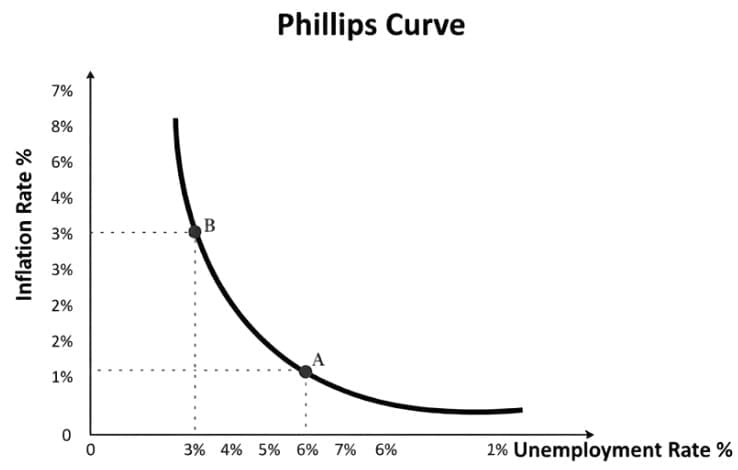
A. W. Phillips published empirical work showing a regular inverse relationship between money wage growth and unemployment rates. His findings suggested that when unemployment is low, wages tend to rise more quickly, and when unemployment is high, wage growth slows.
Economists extended Phillips's wage relationship to a relationship between price inflation and unemployment, arguing that quicker wage growth tends to pass through into higher price inflation. The relationship appeared robust in cross‐country and time‐series evidence in the 1950s and 1960s, but later decades revealed circumstances in which the relationship broke down or shifted, particularly when expectations or supply conditions changed.
The Phillips Curve Relationship - Intuition and Mechanism
- Demand‐driven channel: An increase in aggregate demand raises real output and employment, reducing unemployment.
- Wage pressure: With lower unemployment, the labour market tightens and workers have greater bargaining power, leading to faster wage growth.
- Price pass‐through: Higher wages raise firms' costs and can be passed into higher prices, producing higher inflation.
- Capacity constraints: As the economy approaches full capacity, additional demand primarily increases prices rather than output, strengthening inflationary pressures.
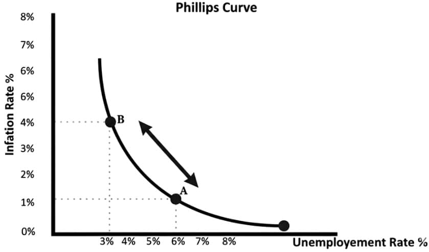
In this simple story, policymakers face a short‐run trade‐off: boosting demand can reduce unemployment but will tend to raise inflation.
Wage Phillips Curve versus Inflation Phillips Curve
- Wage Phillips Curve: The original empirical relationship observed by Phillips was between money wage growth and unemployment.
- Inflation Phillips Curve: Later work and policy discussions focus on consumer price inflation (CPI) or other price indexes versus unemployment, which is more directly relevant for inflation targeting.
Why a Trade‐off Can Appear
The trade‐off emerges because movements in aggregate demand change how tight the labour market is and therefore change wage and price setting behaviour.
Key elements are:
- Labour market tightness: Lower unemployment increases bargaining power for workers and raises the probability of wage rises and job switching.
- Wage‐price interaction: Rising wages raise firms' costs and can lead to price increases when passed on to consumers.
- Expectations: If firms and workers expect higher inflation, they will set wages and prices accordingly, which can either amplify or offset the initial effect.
Monetarist Critique and Expectations
Milton Friedman and Edmund Phelps introduced expectations into the Phillips curve framework and argued the following:
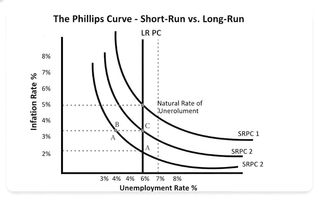
- The economy has a natural rate of unemployment (or NAIRU) determined by labour market structure and supply factors; this is the unemployment rate consistent with stable inflation.
- In the short run, if inflation is unexpectedly higher than expected, unemployment may fall below the natural rate as real wages temporarily decline, increasing employment.
- In the long run, once inflation expectations adjust, the unemployment rate returns to the natural rate and the Phillips curve is vertical: there is no long‐run trade‐off between inflation and unemployment.
- Consequently, attempts to permanently lower unemployment by accepting higher inflation merely raise inflation without improving long‐run unemployment.
Adaptive versus Rational Expectations
- Adaptive expectations: Economic agents form expectations based on past inflation; therefore, there can be a temporary trade‐off until expectations catch up.
- Rational expectations: Agents use all available information and the model of the economy to form expectations; credible policy or anticipated inflation will be incorporated immediately, potentially eliminating even the short‐run trade‐off.
Monetarist View of Aggregate Demand and Aggregate Supply
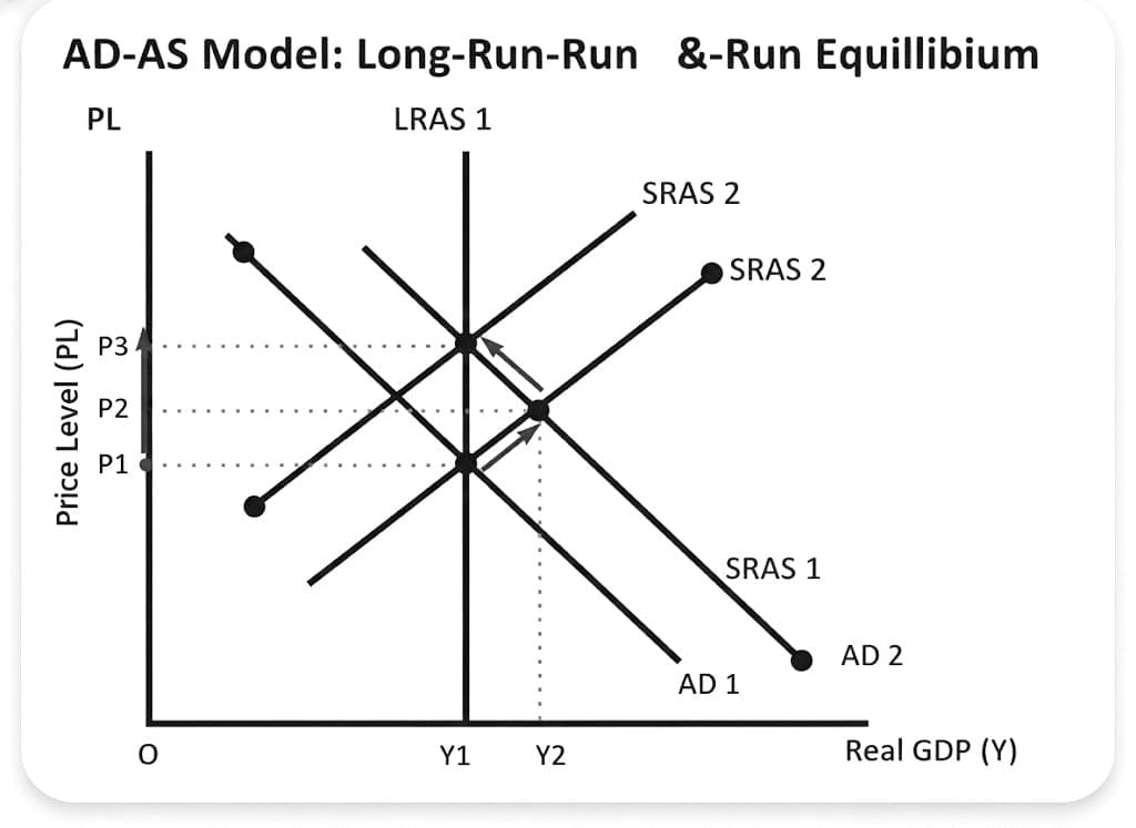
From the monetarist perspective, an increase in aggregate demand (AD) produces a short‐run rise in real output and employment, moving the economy from a point with higher unemployment and lower inflation to one with lower unemployment and higher inflation. Over time, as inflation expectations rise, the short‐run aggregate supply (SRAS) curve shifts left, real output returns toward potential output and unemployment returns toward the natural rate, but inflation is higher than before.
Thus a permanent increase in AD leads only to permanently higher inflation, not permanently lower unemployment.
Keynesian View and Summary of Differences
- Keynesian position: Unemployment can be demand‐deficient and persistent; active demand‐management (fiscal/monetary) can reduce unemployment for a substantial period, especially when there is a large negative output gap.
- Monetarist position: Unemployment is primarily a supply‐side phenomenon; demand management can only reduce unemployment temporarily, and sustained reduction requires supply‐side reforms.
The Phillips Curve Breakdown and Stagflation
In the 1970s many economies experienced stagflation - simultaneous high inflation and high unemployment. This phenomenon appeared to contradict the simple inverse Phillips curve and highlighted the role of:
- Supply shocks: Events such as the oil price shocks of the 1970s raised production costs and shifted supply curves, producing higher inflation and lower output simultaneously.
- Expectations shifts: If inflation expectations rise, the Phillips curve shifts, so the previous trade‐off no longer holds.
The stagflation experience led to greater emphasis on expectations, supply factors and the limits of demand‐management policies.
Empirical Evidence and Modern Perspectives
- NAIRU and measurement: The natural rate of unemployment is not directly observable and estimates can change over time with structural changes in the labour market.
- Flattening of the Phillips curve: Recent decades have seen periods where the empirical relationship between unemployment and inflation has been weak or flatter, influenced by globalisation, anchored expectations, and structural changes in labour markets.
- Policy credibility: Central banks that credibly target low inflation can keep inflation expectations anchored, reducing the short‐run inflationary cost of small deviations in unemployment.
- Role of supply factors: Productivity, labour market institutions, and external shocks can shift the relationship between inflation and unemployment.
Policy Implications
- Policymakers must recognise that any trade‐off between inflation and unemployment is likely to be temporary unless supply conditions change.
- Managing expectations is central: credible inflation targeting reduces the cost of stabilising output and unemployment.
- Supply‐side reforms (labour market flexibility, training, productivity improvements) help reduce the natural rate of unemployment.
- During deep recessions with a large output gap, demand‐management (fiscal or monetary expansion) can reduce unemployment without immediate large inflationary costs; however, sustained demand stimulation risks higher inflation if the economy is near capacity.
Conclusion
The Phillips curve provides a useful framework to think about the interaction between inflation, unemployment and expectations. Historically, it highlighted a perceived trade‐off in the short run, but theoretical developments and empirical experience have shown that the trade‐off is not stable. Expectations, supply shocks and structural factors matter. Policymakers aiming for low inflation and low unemployment should combine credible monetary policy, appropriate demand management when necessary, and supply‐side measures to reduce structural unemployment.
FAQs on Unemployment - Phillips Curve Analysis
| 1. What is the Phillips Curve and its significance in economics? |  |
| 2. What are the main criticisms of the Phillips Curve from the monetarist perspective? | |
| 3. How do Keynesian economists differ from monetarists regarding aggregate demand and supply? | |
| 4. What caused the breakdown of the Phillips Curve during periods of stagflation? | |
| 5. What are the modern perspectives on the Phillips Curve and its policy implications? | |