Forecasting Techniques

Table of Contents
1. Regression Analysis Basics
2. Time-Series Analysis
3. Moving Averages
4. Learning Curves
5. Capital Budgeting Introduction
6. Net Present Value (NPV)
7. Internal Rate of Return (IRR)
8. Payback Period
9. Profitability Index (PI)
10. Integrated Capital Budgeting Example
11. Exam-Specific Questions and Solutions
View more

Forecasting is a critical analytical tool in business decision-making that uses historical data and statistical techniques to predict future outcomes. For CPA candidates, mastering forecasting methods is essential for financial planning, budgeting, and capital investment analysis. This topic bridges quantitative analysis with practical business applications, forming the foundation for evaluating project viability and resource allocation decisions.

1. Regression Analysis Basics

Regression analysis is a statistical method used to establish relationships between variables and predict future values based on historical patterns.

1.1 Simple Linear Regression

Simple Linear Regression examines the relationship between one independent variable (x) and one dependent variable (y). It produces a straight-line equation that best fits the data points.

• Regression Equation: y = a + bx, where y is the dependent variable (what you're predicting), x is the independent variable (predictor), a is the y-intercept (value of y when x = 0), and b is the slope (rate of change in y for each unit change in x)
• Slope Formula: b = [nΣxy - (Σx)(Σy)] / [nΣx² - (Σx)²], where n is the number of observations
• Y-Intercept Formula: a = (Σy/n) - b(Σx/n) or a = ȳ - bx̄, where ȳ is mean of y values and x̄ is mean of x values
• Coefficient of Determination (R²): Measures the percentage of variation in y explained by x. R² ranges from 0 to 1 (0% to 100%). Higher R² indicates better predictive power

1.2 High-Low Method

The High-Low Method is a simplified cost estimation technique that uses only the highest and lowest activity levels to determine the variable cost per unit and fixed cost component.

• Variable Cost per Unit: b = (Cost at High Activity - Cost at Low Activity) / (High Activity Level - Low Activity Level)
• Fixed Cost: a = Total Cost at High Activity - (b × High Activity Level) OR Total Cost at Low Activity - (b × Low Activity Level)
• Limitation: Uses only two data points, ignoring all other observations. May not be representative if outliers are present
• Exam Tip: Always verify which is the high and low activity level (units, hours), not necessarily the high and low cost

1.3 Correlation vs. Causation

• Correlation Coefficient (r): Measures strength and direction of linear relationship between variables. Ranges from -1 to +1. Perfect positive correlation = +1, perfect negative correlation = -1, no correlation = 0
• Trap Alert: Strong correlation does NOT imply causation. Two variables may move together due to a third factor or pure coincidence
• Standard Error of Estimate: Measures the dispersion of actual values around the regression line. Lower standard error indicates better predictive accuracy

2. Time-Series Analysis

Time-series analysis examines data points collected at successive time intervals to identify patterns and forecast future values.

2.1 Components of Time-Series Data

• Trend (T): Long-term upward or downward movement in data over time. Represents the underlying direction of the series
• Seasonality (S): Regular, predictable patterns that repeat over fixed periods (quarterly, monthly, weekly). Examples include retail sales peaks during holidays, utility usage variations by season
• Cyclical Variations (C): Fluctuations lasting more than one year, often tied to economic or business cycles. Differ from seasonality because cycles are irregular and longer
• Irregular/Random Component (I): Unpredictable, erratic movements caused by unexpected events (natural disasters, strikes, sudden policy changes)

2.2 Time-Series Models

• Additive Model: Y = T + S + C + I. Used when seasonal variations remain relatively constant in absolute terms regardless of trend level
• Multiplicative Model: Y = T × S × C × I. Used when seasonal variations change proportionally with the trend level. More common in business applications
• Deseasonalizing Data: Process of removing seasonal component to reveal underlying trend. Formula: Deseasonalized Value = Actual Value / Seasonal Index (for multiplicative model)

2.3 Seasonal Index Calculation

1. Step 1: Calculate the average for each season across all years in the dataset
2. Step 2: Calculate the grand average (overall mean of all observations)
3. Step 3: Seasonal Index = (Average for Season / Grand Average) × 100 (expressed as percentage or ratio)
4. Verification Check: Sum of all seasonal indices should equal number of seasons × 100 (or number of seasons if expressed as ratios)

3. Moving Averages

Moving averages smooth out short-term fluctuations to reveal underlying trends and patterns in time-series data.

3.1 Simple Moving Average (SMA)

The Simple Moving Average calculates the average of a fixed number of recent periods, with each period weighted equally.

• Formula: SMA = (Sum of n Most Recent Observations) / n, where n is the number of periods included
• 3-Period Moving Average: Most common for quarterly data. Averages current period and two preceding periods
• 4-Period Moving Average: Typically used for monthly data to identify quarterly patterns
• Data Points Lost: With an n-period moving average, you lose (n-1) data points at the beginning of the series
• Lag Effect: Moving averages lag behind actual changes because they include historical data. Longer periods create greater lag

3.2 Weighted Moving Average (WMA)

The Weighted Moving Average assigns different weights to observations, typically giving more importance to recent data.

• Formula: WMA = (w₁x₁ + w₂x₂ + ... + wₙxₙ) / (w₁ + w₂ + ... + wₙ), where w represents weights and x represents observed values
• Weight Assignment: Most recent period receives highest weight, declining for older periods. Weights must be disclosed or specified in the problem
• Advantage over SMA: More responsive to recent changes while still smoothing fluctuations
• Exam Tip: Always verify that weights sum to the denominator used. Some problems express weights as decimals that sum to 1.0

3.3 Exponential Smoothing

Exponential Smoothing is a sophisticated weighted average method where weights decrease exponentially for older observations.

• Formula: F_t+1 = αA_t + (1-α)F_t, where F_t+1 is the forecast for next period, A_t is the actual value in current period, F_t is the forecast for current period, and α is the smoothing constant (0 < α=""><>
• Alternative Form: F_t+1 = F_t + α(A_t - F_t). This shows the forecast adjusts by a fraction of the forecast error
• Smoothing Constant (α): Higher α (0.5 to 1.0) = more weight on recent data, more responsive to changes. Lower α (0.1 to 0.3) = more smoothing, less responsive
• Initial Forecast: When no prior forecast exists, use the first actual observation or an average of early observations as F₁
• Trap Alert: Don't confuse A (actual) with F (forecast). The formula updates the forecast based on the error between actual and forecasted values

4. Learning Curves

Learning curves (also called Experience Curves) reflect the principle that unit costs decline predictably as cumulative production increases due to worker efficiency gains and process improvements.

4.1 Learning Curve Concept

• Learning Curve Rate: The percentage of the prior cost that the cumulative average cost per unit falls to when production doubles. Common rates: 80%, 75%, 70%
• 80% Learning Curve: When output doubles, cumulative average time (or cost) per unit = 80% of what it was before doubling
• Application Areas: Labor-intensive manufacturing, assembly operations, new product launches, employee training programs
• Assumptions: No production interruptions, consistent production methods, motivated workforce, complex or repetitive tasks

4.2 Cumulative Average-Time Learning Model

This is the most commonly tested learning curve model for CPA exams.

• Formula: Y = aX^b, where Y is cumulative average time per unit, a is time required for first unit, X is cumulative number of units produced, and b is the learning index
• Learning Index (b): b = log(learning rate) / log(2). For 80% curve: b = log(0.80) / log(2) = -0.3219
• Doubling Rule: Every time cumulative production doubles, cumulative average time per unit = previous average × learning rate
• Total Time Calculation: Total Time for X Units = Cumulative Average Time per Unit × X
• Incremental Time: Time for units from X₁ to X₂ = (Total Time for X₂) - (Total Time for X₁)

4.3 Learning Curve Tables

CPA exam problems typically provide learning curve tables showing cumulative average time coefficients for different production levels.

• Table Usage: Locate the intersection of cumulative units and learning rate percentage. Multiply the coefficient by the time for the first unit
• Example Coefficients (80% curve): 1 unit = 1.0000, 2 units = 0.8000, 4 units = 0.6400, 8 units = 0.5120, 16 units = 0.4096
• Verification Pattern: Each doubling multiplies the prior coefficient by the learning rate (0.8000 = 1.0000 × 0.80; 0.6400 = 0.8000 × 0.80)

4.4 Common Learning Curve Pitfalls

• Trap Alert: Learning curve coefficients represent cumulative average time, NOT the time for individual units. Don't multiply the coefficient directly by the number of units to get total time
• Trap Alert: The learning rate applies only when production doubles (1→2→4→8→16). For non-doubling quantities, use tables or formulas
• Steady State: Learning effect diminishes after production reaches high volumes. Eventually, time per unit levels off

5. Capital Budgeting Introduction

Capital budgeting is the process of evaluating and selecting long-term investments that align with the firm's goal of maximizing shareholder wealth. These decisions involve substantial cash outflows and generate returns over multiple years.

5.1 Capital Budgeting Framework

• Characteristics of Capital Projects: Large initial investment, long-term impact (multiple years), irreversible or costly to reverse, strategic importance to organization
• Project Classification: Independent projects (acceptance of one doesn't affect others), mutually exclusive projects (accepting one precludes others), contingent projects (depend on acceptance of another project)
• Cash Flow Focus: Capital budgeting uses cash flows, not accounting income. Ignore non-cash expenses like depreciation for cash flow analysis, but consider depreciation's tax shield effect
• Relevant Cash Flows: Include only incremental cash flows directly attributable to the project. Exclude sunk costs (already incurred), ignore allocated overhead unless it increases

5.2 Time Value of Money Foundation

• Present Value (PV): Current worth of future cash flows discounted at an appropriate rate. Formula: PV = FV / (1+r)ⁿ, where FV is future value, r is discount rate, n is number of periods
• Future Value (FV): Amount an investment will grow to over time. Formula: FV = PV × (1+r)ⁿ
• Discount Rate Selection: Typically the firm's cost of capital (WACC) or required rate of return. Reflects the opportunity cost of capital and project risk
• Annuity: Series of equal cash flows at regular intervals. PV of Ordinary Annuity = PMT × [(1 - (1+r)⁻ⁿ) / r], where PMT is periodic payment

5.3 Capital Budgeting Methods Overview

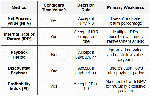
6. Net Present Value (NPV)

NPV is the most theoretically sound capital budgeting method. It measures the dollar amount by which a project increases or decreases firm value.

6.1 NPV Calculation

• NPV Formula: NPV = Σ [CF_t / (1+r)ᵗ] - Initial Investment, where CF_t is cash flow in period t, r is discount rate (cost of capital), t is time period
• Alternative Expression: NPV = PV of Future Cash Inflows - PV of Cash Outflows (including initial investment)
• Decision Rule: Accept project if NPV > 0 (adds value), reject if NPV < 0="" (destroys="" value),="" indifferent="" if="" npv="0">
• Ranking Projects: For mutually exclusive projects, select the project with the highest positive NPV

6.2 NPV Computation Steps

1. Identify all relevant cash flows: Initial investment (usually negative), annual operating cash flows, terminal cash flows (salvage value, working capital recovery)
2. Determine the appropriate discount rate: Use cost of capital or required rate of return adjusted for project risk
3. Calculate present value of each cash flow: Multiply each cash flow by the appropriate present value factor or use PV formula
4. Sum all present values: Add all discounted cash inflows and subtract all discounted cash outflows
5. Apply decision rule: Accept if NPV is positive

6.3 NPV Advantages and Limitations

• Advantages: Considers time value of money, considers all cash flows over project life, directly measures value creation, additive (NPVs of independent projects can be summed), consistent with shareholder wealth maximization
• Disadvantages: Requires estimation of discount rate, difficult to explain to non-financial managers, absolute dollar measure (doesn't show return percentage), sensitive to discount rate changes
• Trap Alert: Initial investment is already a present value (occurs at t=0). Don't discount it further. Only discount future cash flows
• Unequal Project Lives: When comparing projects with different lifespans, use Equivalent Annual Annuity (EAA) method or Replacement Chain approach

6.4 Tax Effects on NPV

• After-Tax Cash Flows: Operating Cash Flow = (Revenues - Cash Expenses) × (1 - Tax Rate) + (Depreciation × Tax Rate)
• Depreciation Tax Shield: Depreciation itself isn't a cash flow, but it reduces taxable income. Tax savings = Depreciation × Tax Rate
• Salvage Value: If asset sells for more than book value, tax is owed on the gain. If less than book value, tax loss creates savings
• Working Capital: Increases in working capital are cash outflows; recovery at project end is cash inflow. Both affect NPV

7. Internal Rate of Return (IRR)

IRR is the discount rate that makes the NPV of a project equal to zero. It represents the expected compound annual rate of return from the project.

7.1 IRR Concept and Calculation

• IRR Definition: The rate (r) that satisfies: Σ [CF_t / (1+r)ᵗ] - Initial Investment = 0, or equivalently, PV of Inflows = PV of Outflows
• Decision Rule: Accept project if IRR > required rate of return (cost of capital), reject if IRR < required="" rate="" of="">
• Calculation Methods: Trial and error using PV tables, financial calculator (enter CF₀, CF₁, CF₂,... then compute IRR), spreadsheet functions (Excel: =IRR(values))
• Interpolation: If using tables, calculate NPV at two discount rates. IRR lies between the rate giving positive NPV and the rate giving negative NPV

7.2 IRR Interpolation Formula

When NPV is positive at rate r₁ and negative at rate r₂:

• IRR Formula: IRR = r₁ + [NPV₁ / (NPV₁ - NPV₂)] × (r₂ - r₁), where r₁ is lower rate with positive NPV, r₂ is higher rate with negative NPV, NPV₁ is positive NPV at r₁, NPV₂ is negative NPV at r₂ (use absolute values in calculation)
• Exam Tip: Choose r₁ and r₂ close together (differ by 1-2%) for more accurate interpolation

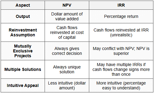
7.3 IRR vs. NPV Comparison

7.4 IRR Problems and Limitations

• Multiple IRRs: Projects with non-conventional cash flows (multiple sign changes) may have multiple IRRs or no real IRR. Example: Initial outflow, then inflows, then another outflow
• Scale Problem: IRR doesn't consider project size. A small project with 25% IRR may be less valuable than large project with 20% IRR
• Timing Problem: IRR may favor projects with earlier cash flows even if later-cash-flow projects have higher NPV
• Ranking Conflicts: For mutually exclusive projects, IRR and NPV may rank projects differently. Always use NPV for final decision
• Trap Alert: Don't confuse IRR with required rate of return. IRR is what you earn; required rate is what you need to earn

7.5 Modified Internal Rate of Return (MIRR)

MIRR addresses IRR's reinvestment rate assumption by assuming cash flows are reinvested at the cost of capital.

• MIRR Calculation: Find terminal value of cash inflows compounded at cost of capital. Find PV of cash outflows at cost of capital. MIRR is the rate equating these two values
• MIRR Formula: MIRR = [(Terminal Value of Inflows / PV of Outflows)^(1/n)] - 1, where n is project life in years
• Advantages: Unique solution always exists, more realistic reinvestment assumption, better for comparing projects than IRR

8. Payback Period

Payback period measures how long it takes for a project's cumulative cash flows to equal its initial investment. It focuses on liquidity and risk rather than profitability.

8.1 Simple Payback Period

• Definition: Number of years required to recover the initial cash investment from project cash flows (ignoring time value of money)
• Even Cash Flows: Payback Period = Initial Investment / Annual Cash Flow
• Uneven Cash Flows: Cumulative method - Add annual cash flows until cumulative total equals initial investment. If recovery falls between years, calculate fractional year
• Fractional Year: If year n has cumulative CF less than investment and year n+1 exceeds it: Payback = n + (Remaining Amount Needed / Cash Flow in Year n+1)
• Decision Rule: Accept if payback period ≤ company's maximum acceptable payback period. Shorter payback is better

8.2 Discounted Payback Period

Discounted payback improves on simple payback by incorporating time value of money.

• Method: Calculate present value of each year's cash flow using the required rate of return. Sum discounted cash flows cumulatively until initial investment is recovered
• Comparison: Discounted payback is always longer than simple payback because future cash flows are worth less in present value terms
• Advantage over Simple Payback: Considers time value of money, making it more economically sound

8.3 Payback Advantages and Limitations

• Advantages: Simple to calculate and understand, provides liquidity measure, useful for risky projects or industries with rapid technological change, emphasizes quick return of capital
• Major Limitations: Ignores time value of money (simple version), ignores all cash flows after payback period (may reject profitable long-term projects), ignores project profitability, no objective criterion for maximum acceptable payback
• Trap Alert: Projects with shorter payback aren't necessarily more profitable. A project recovering investment in 3 years might be less valuable than one taking 5 years if the latter has much larger total cash flows
• Bias: Payback favors short-term projects and may cause underinvestment in long-term value-creating opportunities

9. Profitability Index (PI)

The profitability index (also called Benefit-Cost Ratio) measures the present value of benefits per dollar of investment. It's particularly useful when capital is rationed.

9.1 PI Calculation and Decision Rule

• PI Formula: PI = PV of Future Cash Inflows / Initial Investment (or PV of Cash Outflows)
• Alternative Formula: PI = (NPV + Initial Investment) / Initial Investment = 1 + (NPV / Initial Investment)
• Decision Rule: Accept project if PI > 1.0 (equivalent to NPV > 0), reject if PI < 1.0="" (equivalent="" to="" npv="">< 0),="" indifferent="" if="" pi="1.0" (equivalent="" to="" npv="">
• Interpretation: PI = 1.25 means the project returns $1.25 in present value for every $1.00 invested

9.2 PI Applications

• Capital Rationing: When investment funds are limited, rank independent projects by PI. Select projects with highest PI until budget is exhausted
• Efficiency Measure: PI shows bang-for-buck - which projects provide most value per dollar invested
• Advantage over NPV: Better for comparing projects of different sizes under capital constraints
• Trap Alert: For mutually exclusive projects not under capital rationing, PI may give wrong decision. Use NPV instead

9.3 Ranking Conflicts

• NPV vs. PI Conflict: When choosing between mutually exclusive projects, NPV and PI may rank them differently
• Example: Project A: Investment $100, NPV $50, PI = 1.50. Project B: Investment $500, NPV $180, PI = 1.36. PI favors A; NPV favors B
• Resolution: If no capital rationing exists, choose Project B (higher NPV adds more value). If capital is constrained, PI provides better guidance
• Exam Tip: Always check whether the problem mentions capital rationing or budget constraints before selecting decision criterion

10. Integrated Capital Budgeting Example

A comprehensive example demonstrates how different methods apply to the same project and shows why conclusions may differ.

10.1 Sample Problem Setup

Given Data: Initial Investment = $100,000, Project Life = 5 years, Annual Cash Inflows: Year 1 = $25,000, Year 2 = $30,000, Year 3 = $35,000, Year 4 = $30,000, Year 5 = $25,000, Required Rate of Return = 10%, Salvage Value = $0

10.2 Solution Using All Methods

NPV Calculation:

• PV Year 1 = $25,000 / (1.10)¹ = $22,727
• PV Year 2 = $30,000 / (1.10)² = $24,793
• PV Year 3 = $35,000 / (1.10)³ = $26,296
• PV Year 4 = $30,000 / (1.10)⁴ = $20,490
• PV Year 5 = $25,000 / (1.10)⁵ = $15,523
• Total PV of Inflows = $109,829
• NPV = $109,829 - $100,000 = $9,829 (Accept - positive NPV)

IRR Calculation:

• Using financial calculator or Excel: IRR ≈ 12.6%
• Decision: Accept because 12.6% > 10% required rate

Payback Period:

• Cumulative CF Year 1 = $25,000
• Cumulative CF Year 2 = $55,000
• Cumulative CF Year 3 = $90,000
• Cumulative CF Year 4 = $120,000 (exceeds $100,000)
• Payback = 3 + [($100,000 - $90,000) / $30,000] = 3.33 years
• Decision: Accept if company's maximum acceptable payback > 3.33 years

Profitability Index:

• PI = $109,829 / $100,000 = 1.098
• Decision: Accept because PI > 1.0

10.3 Common Student Mistakes

• Mistake 1: Forgetting to subtract initial investment after calculating PV of inflows when computing NPV
• Mistake 2: Discounting the initial investment (Year 0 cash flow is already at present value)
• Mistake 3: Using IRR to choose between mutually exclusive projects without checking NPV
• Mistake 4: Calculating payback using discounted cash flows when problem asks for simple payback
• Mistake 5: Including sunk costs or allocated overhead that doesn't change with the project
• Mistake 6: Forgetting depreciation tax shield when calculating after-tax cash flows
• Mistake 7: Using accounting income instead of cash flows for capital budgeting analysis

11. Exam-Specific Questions and Solutions

11.1 Regression Analysis Question

Question: A company collected the following data on maintenance costs and machine hours over six months:

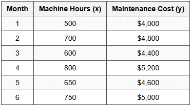
Using the high-low method, what is the variable cost per machine hour and fixed cost component?

Solution:

• Step 1 - Identify High and Low Activity Levels: High = 800 hours with $5,200 cost, Low = 500 hours with $4,000 cost
• Step 2 - Calculate Variable Cost: b = ($5,200 - $4,000) / (800 - 500) = $1,200 / 300 = $4.00 per machine hour
• Step 3 - Calculate Fixed Cost: Using high point: a = $5,200 - ($4.00 × 800) = $5,200 - $3,200 = $2,000
• Verification using low point: a = $4,000 - ($4.00 × 500) = $4,000 - $2,000 = $2,000 ✓
• Cost Formula: y = $2,000 + $4.00x
• Answer: Variable cost = $4.00 per machine hour; Fixed cost = $2,000

11.2 Moving Average Question

Question: Quarterly sales data (in thousands): Q1 = $120, Q2 = $140, Q3 = $160, Q4 = $180, Q5 = $150. Calculate a 3-quarter moving average for Q4 and Q5.

Solution:

• Q4 Moving Average: (Q2 + Q3 + Q4) / 3 = ($140 + $160 + $180) / 3 = $480 / 3 = $160
• Q5 Moving Average: (Q3 + Q4 + Q5) / 3 = ($160 + $180 + $150) / 3 = $490 / 3 = $163.33
• Answer: Q4 moving average = $160,000; Q5 moving average = $163,333

11.3 Learning Curve Question

Question: The first unit of a product requires 100 hours to produce. The company experiences an 80% learning curve. How many hours will be required to produce the 4th unit on a cumulative average basis? What is the total time for all 4 units?

Solution:

• Step 1 - Apply Doubling Rule: 1st unit = 100 hours (cumulative average = 100). 2 units cumulative average = 100 × 0.80 = 80 hours. 4 units cumulative average = 80 × 0.80 = 64 hours
• Step 2 - Calculate Total Time: Total time for 4 units = Cumulative average × Number of units = 64 hours × 4 = 256 hours
• Answer: Cumulative average time for 4 units = 64 hours per unit; Total time for all 4 units = 256 hours
• Key Point: The 64 hours is the average per unit for all 4 units, not the time for just the 4th unit

11.4 NPV Question

Question: A project requires initial investment of $50,000. It will generate after-tax cash flows of $15,000 per year for 5 years. The company's cost of capital is 12%. Should the project be accepted?

Solution:

• Step 1 - Recognize Annuity: Equal annual cash flows = ordinary annuity
• Step 2 - Find PV Factor: PV annuity factor for 5 years at 12% = 3.605 (from PV tables)
• Step 3 - Calculate PV of Inflows: PV = $15,000 × 3.605 = $54,075
• Step 4 - Calculate NPV: NPV = $54,075 - $50,000 = $4,075
• Decision: Accept the project because NPV > 0. The project adds $4,075 to firm value

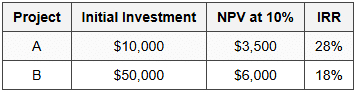
11.5 IRR vs. NPV Conflict Question

Question: Two mutually exclusive projects have the following characteristics at 10% discount rate:

Which project should be selected and why?

Solution:

• Conflict Identification: IRR favors Project A (28% > 18%), but NPV favors Project B ($6,000 > $3,500)
• Analysis: Projects are mutually exclusive, so only one can be selected. No capital rationing mentioned
• Correct Decision: Select Project B based on NPV criterion
• Reasoning: NPV is superior for mutually exclusive projects. Project B adds more absolute value to the firm ($6,000 vs. $3,500)
• Why IRR Misleads: IRR doesn't account for scale differences. Project A's higher percentage return applies to much smaller investment
• Answer: Choose Project B; it creates $2,500 more value than Project A despite lower percentage return

11.6 Profitability Index - Capital Rationing Question

Question: A company has $100,000 to invest and faces the following independent projects (all have 3-year lives):

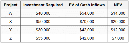
Which combination of projects should be selected?

Solution:

• Step 1 - Calculate PI for Each Project:
  • Project W: PI = $54,000 / $40,000 = 1.35
  • Project X: PI = $70,000 / $50,000 = 1.40
  • Project Y: PI = $42,000 / $30,000 = 1.40
  • Project Z: PI = $42,000 / $35,000 = 1.20
• Step 2 - Rank by PI: Projects X and Y tied at 1.40 (highest), W at 1.35, Z at 1.20 (lowest)
• Step 3 - Select Projects: X ($50,000) + Y ($30,000) = $80,000 total investment (within $100,000 budget)
• Step 4 - Check if Adding More: Remaining budget = $20,000. Neither W ($40,000) nor Z ($35,000) fits
• Alternative Check: W + Y = $70,000 investment, NPV = $26,000. X + Y = $80,000 investment, NPV = $32,000 (better)
• Answer: Select Projects X and Y. Total investment = $80,000; Total NPV = $32,000
• Key Learning: Under capital rationing, PI provides better ranking than NPV alone. Focus on value per dollar invested

11.7 Exponential Smoothing Question

Question: Actual demand for January = 200 units. The forecast for January was 180 units. Using a smoothing constant (α) of 0.3, what is the forecast for February?

Solution:

• Given: F₁ (Jan forecast) = 180, A₁ (Jan actual) = 200, α = 0.3
• Formula: F₂ = αA₁ + (1-α)F₁
• Calculation: F₂ = (0.3 × 200) + (0.7 × 180) = 60 + 126 = 186 units
• Alternative Method: F₂ = F₁ + α(A₁ - F₁) = 180 + 0.3(200 - 180) = 180 + 6 = 186 units
• Interpretation: Forecast adjusts upward by 30% of the forecast error (20 units), increasing from 180 to 186
• Answer: February forecast = 186 units

11.8 Payback with Uneven Cash Flows Question

Question: Initial investment = $80,000. Annual cash flows: Year 1 = $20,000, Year 2 = $25,000, Year 3 = $30,000, Year 4 = $35,000. Calculate the payback period.

Solution:

• Cumulative CF Year 1: $20,000
• Cumulative CF Year 2: $20,000 + $25,000 = $45,000
• Cumulative CF Year 3: $45,000 + $30,000 = $75,000
• Cumulative CF Year 4: $75,000 + $35,000 = $110,000 (exceeds $80,000 investment)
• Payback Calculation: Investment recovered between Years 3 and 4. Amount still needed after Year 3 = $80,000 - $75,000 = $5,000
• Fractional Year: $5,000 / $35,000 = 0.143 years
• Answer: Payback Period = 3.14 years (or 3 years, 1.7 months)

11.9 Learning Curve Incremental Time Question

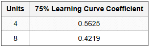
Question: A company operates under a 75% learning curve. The first unit requires 40 hours. Using the table below, how many hours will units 5 through 8 require in total?

Solution:

• Step 1 - Calculate Total Time for 8 Units: Cumulative average for 8 units = 40 hours × 0.4219 = 16.876 hours per unit. Total time for 8 units = 16.876 × 8 = 135.01 hours
• Step 2 - Calculate Total Time for First 4 Units: Cumulative average for 4 units = 40 hours × 0.5625 = 22.5 hours per unit. Total time for 4 units = 22.5 × 4 = 90 hours
• Step 3 - Calculate Incremental Time: Time for units 5-8 = Total for 8 units - Total for 4 units = 135.01 - 90 = 45.01 hours
• Answer: Units 5 through 8 will require approximately 45 hours in total
• Key Concept: To find time for specific unit range, subtract cumulative totals

11.10 Comprehensive Capital Budgeting Question

Question: A company is evaluating a 4-year project with the following information: Initial equipment cost = $200,000, Installation cost = $20,000, Annual revenues = $150,000, Annual cash expenses = $60,000, Depreciation (straight-line) = $55,000 per year, Tax rate = 30%, Required return = 14%, Working capital required at start = $30,000 (fully recovered at end), Salvage value = $0. Calculate the NPV.

Solution:

• Step 1 - Initial Investment: Equipment + Installation + Working Capital = $200,000 + $20,000 + $30,000 = $250,000
• Step 2 - Annual Operating Cash Flow:
  • Revenues: $150,000
  • Cash Expenses: ($60,000)
  • Depreciation: ($55,000) - non-cash but affects taxes
  • Operating Income (before tax): $35,000
  • Tax (30%): ($10,500)
  • After-tax Income: $24,500
  • Add back Depreciation: $55,000
  • Operating Cash Flow = $79,500 per year
• Alternative OCF Formula: OCF = (Rev - Cash Exp)(1-T) + (Dep × T) = ($150,000 - $60,000)(0.70) + ($55,000 × 0.30) = $63,000 + $16,500 = $79,500 ✓
• Step 3 - Terminal Cash Flow: Working capital recovery in Year 4 = $30,000
• Step 4 - Total Cash Flow Year 4: $79,500 + $30,000 = $109,500
• Step 5 - PV Calculations at 14%:
  • PV Year 1: $79,500 / 1.14 = $69,737
  • PV Year 2: $79,500 / (1.14)² = $61,173
  • PV Year 3: $79,500 / (1.14)³ = $53,661
  • PV Year 4: $109,500 / (1.14)⁴ = $64,860
  • Total PV of Inflows = $249,431
• Step 6 - Calculate NPV: NPV = $249,431 - $250,000 = -$569
• Decision: Reject the project (NPV < 0,="" though="">
• Answer: NPV = -$569; Recommendation: Reject

Mastering forecasting techniques and capital budgeting methods is essential for CPA candidates tackling the Business Analysis section. These tools form the quantitative foundation for strategic business decisions. Remember that NPV is theoretically superior for project selection, though understanding all methods and their limitations is crucial for comprehensive analysis. Practice applying these formulas systematically, pay attention to the specific requirements of each question, and always verify your calculations. Focus on understanding the economic intuition behind each technique, as this will help you navigate complex scenario-based questions on the exam.