Hypothesis Testing

Table of Contents
1. Fundamentals of Hypothesis Testing
2. Key Concepts in Hypothesis Testing
3. Steps in Hypothesis Testing
4. Common Hypothesis Tests
5. Assumptions and Conditions
6. Parametric vs Non-Parametric Tests
7. Effect Size
8. Confidence Intervals and Hypothesis Testing
9. Multiple Testing Problem
10. Practical Implementation Considerations
11. Common Mistakes and Misconceptions
View more

Hypothesis Testing is a fundamental statistical method used to make decisions or draw conclusions about a population based on sample data. It allows us to test claims, compare groups, and validate assumptions using a structured, mathematical approach. This chapter forms the backbone of inferential statistics and is critical for making data-driven decisions in business analysis, machine learning model evaluation, and scientific research. You will learn how to formulate hypotheses, choose appropriate tests, calculate test statistics, interpret p-values, and draw valid conclusions from data.

1. Fundamentals of Hypothesis Testing

1.1 Definition and Purpose

Hypothesis Testing is a statistical procedure to evaluate whether sample data provides sufficient evidence to reject a claim about a population parameter.

• Purpose: To make objective decisions about population characteristics when we only have sample data
• Applications: A/B testing in marketing, quality control in manufacturing, clinical trials in medicine, model performance validation in ML
• Foundation: Based on probability theory and sampling distributions

1.2 Null Hypothesis (H₀) and Alternative Hypothesis (H₁ or Hₐ)

Every hypothesis test involves two competing statements about a population parameter:

• Null Hypothesis (H₀): The default assumption or claim of "no effect" or "no difference". It represents the status quo and always contains an equality (=, ≤, or ≥)
• Alternative Hypothesis (H₁): The claim we want to test or prove. It contradicts H₀ and contains inequality (≠, <, or="">)
• Key Rule: We never "accept" H₀; we only "fail to reject" it or "reject" it in favor of H₁

Example: Testing if a new drug reduces blood pressure:

• H₀: The drug has no effect (mean difference = 0)
• H₁: The drug reduces blood pressure (mean difference <>

1.3 Types of Hypothesis Tests

Based on the direction of the alternative hypothesis:

1. Two-tailed test: H₁ states the parameter is not equal to a value (≠). Tests for difference in either direction. Example: H₀: μ = 100 vs H₁: μ ≠ 100
2. Right-tailed test: H₁ states the parameter is greater than a value (>). Tests for increase only. Example: H₀: μ ≤ 100 vs H₁: μ > 100
3. Left-tailed test: H₁ states the parameter is less than a value (<). tests="" for="" decrease="" only.="" example:="" h₀:="" μ="" ≥="" 100="" vs="" h₁:="" μ=""><>

2. Key Concepts in Hypothesis Testing

2.1 Test Statistic

A Test Statistic is a standardized value calculated from sample data that measures how far the sample statistic deviates from the null hypothesis value.

• Purpose: Converts sample information into a single number for decision-making
• Common test statistics: z-score, t-statistic, chi-square statistic, F-statistic
• General formula: Test Statistic = (Sample Statistic - Hypothesized Parameter) / Standard Error

2.2 Significance Level (α)

The Significance Level (α) is the probability threshold for rejecting H₀ when it is actually true (Type I error rate).

• Common values: α = 0.05 (5%), α = 0.01 (1%), α = 0.10 (10%)
• Standard choice: α = 0.05 means we accept a 5% risk of false positive
• Interpretation: Lower α means stricter criteria for rejecting H₀
• Set before analysis: Must be predetermined, not adjusted based on results

2.3 p-value

The p-value is the probability of obtaining test results at least as extreme as observed, assuming H₀ is true.

• Decision rule: If p-value ≤ α, reject H₀. If p-value > α, fail to reject H₀
• Interpretation: Lower p-value = stronger evidence against H₀
• Not probability of H₀: p-value does NOT tell us the probability that H₀ is true
• Example: p-value = 0.03 with α = 0.05 means we reject H₀

Trap Alert: A common mistake is interpreting p-value as "probability that H₀ is true" or "probability that results occurred by chance." The correct interpretation is: "probability of observing data this extreme if H₀ were true."

2.4 Critical Value and Rejection Region

The Critical Value is the boundary value(s) that separates the rejection region from the non-rejection region.

• Rejection Region: The range of test statistic values that leads to rejecting H₀
• Critical Region approach: Compare test statistic directly with critical value instead of using p-value
• For two-tailed test: Two critical values (one positive, one negative)
• For one-tailed test: One critical value (either positive or negative)

2.5 Types of Errors

Two types of errors can occur in hypothesis testing:

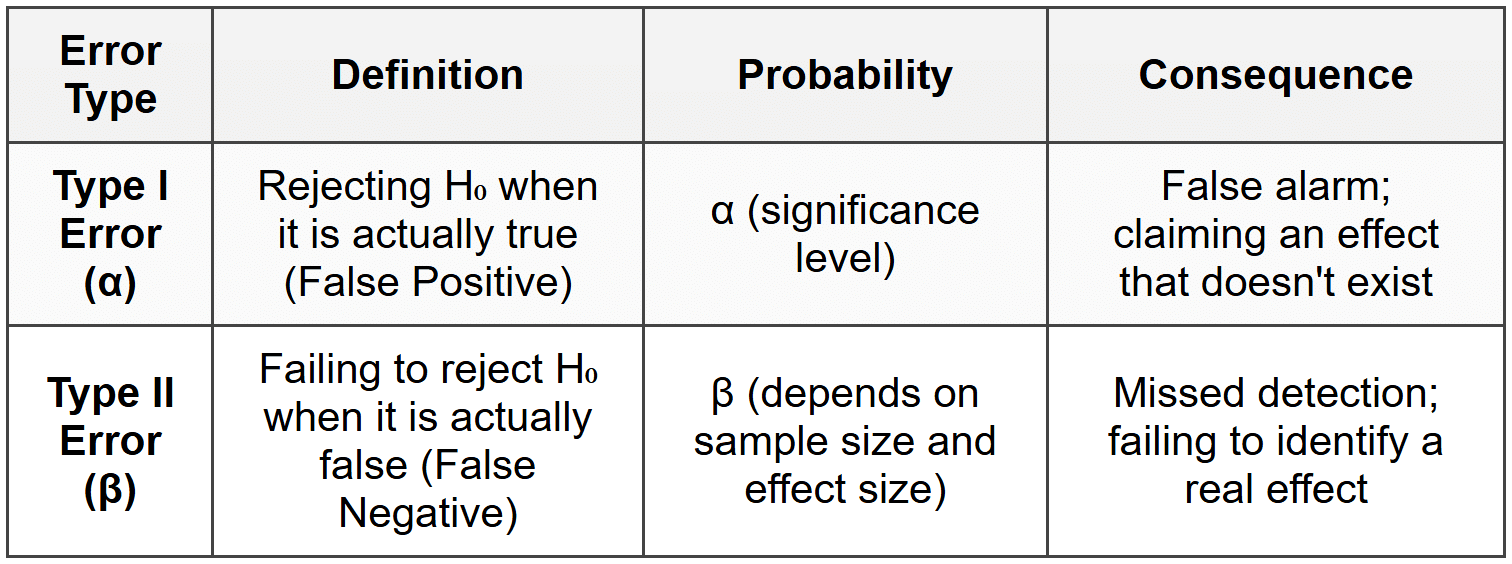
• Trade-off: Decreasing α (stricter test) typically increases β, and vice versa
• Power of test: (1 - β) = probability of correctly rejecting false H₀

2.6 Statistical Power

Statistical Power is the probability of correctly rejecting H₀ when it is false (detecting a true effect).

• Formula: Power = 1 - β
• Desired value: Typically aim for power ≥ 0.80 (80%)
• Factors increasing power: Larger sample size, larger effect size, higher α, lower variability
• Importance: Low power means high risk of missing real effects

3. Steps in Hypothesis Testing

A systematic 5-step process for conducting hypothesis tests:

1. State the Hypotheses: Clearly define H₀ and H₁ based on the research question. Identify if test is one-tailed or two-tailed
2. Choose Significance Level: Set α (typically 0.05). This determines acceptable Type I error rate
3. Select and Calculate Test Statistic: Choose appropriate test based on data type and assumptions. Calculate test statistic from sample data
4. Determine p-value or Critical Value: Find p-value using test statistic distribution OR identify critical value(s) from statistical tables
5. Make Decision and Interpret: Compare p-value with α (or test statistic with critical value). State conclusion in context of original problem

4. Common Hypothesis Tests

4.1 One-Sample Tests

Used when comparing a single sample to a known or hypothesized population value.

4.1.1 One-Sample Z-Test

• Purpose: Test if population mean equals a specific value when population standard deviation (σ) is known
• Requirements: Known σ, normally distributed population OR large sample (n ≥ 30)
• Test Statistic: z = (x̄ - μ₀) / (σ / √n)
• Parameters: x̄ = sample mean, μ₀ = hypothesized population mean, σ = population standard deviation, n = sample size
• Distribution: Standard normal distribution (z-distribution)

4.1.2 One-Sample t-Test

• Purpose: Test if population mean equals a specific value when population standard deviation is unknown
• Requirements: Unknown σ, approximately normal distribution (especially for small samples)
• Test Statistic: t = (x̄ - μ₀) / (s / √n)
• Parameters: x̄ = sample mean, μ₀ = hypothesized mean, s = sample standard deviation, n = sample size
• Degrees of freedom: df = n - 1
• Distribution: Student's t-distribution
• Most common: This is more frequently used than z-test because σ is rarely known in practice

4.2 Two-Sample Tests

Used when comparing means or proportions between two independent groups.

4.2.1 Independent Two-Sample t-Test

• Purpose: Test if means of two independent populations are equal
• Requirements: Two independent samples, approximately normal distributions, similar variances (homogeneity)
• Hypotheses: H₀: μ₁ = μ₂ vs H₁: μ₁ ≠ μ₂ (or < or="">)
• Test Statistic (equal variances): t = (x̄₁ - x̄₂) / (s_pooled × √(1/n₁ + 1/n₂))
• Pooled standard deviation: s_pooled = √[((n₁-1)s₁² + (n₂-1)s₂²) / (n₁+n₂-2)]
• Degrees of freedom: df = n₁ + n₂ - 2
• Welch's t-test: Used when variances are unequal (does not assume equal variances)

4.2.2 Paired t-Test (Dependent Samples)

• Purpose: Test if mean difference between paired observations equals zero
• Use cases: Before-after measurements, matched pairs, repeated measures on same subjects
• Requirements: Paired observations, differences approximately normally distributed
• Test Statistic: t = (d̄ - 0) / (s_d / √n)
• Parameters: d̄ = mean of differences, s_d = standard deviation of differences, n = number of pairs
• Degrees of freedom: df = n - 1

Trap Alert: Students often confuse independent and paired t-tests. Use paired t-test ONLY when observations are naturally paired (same subject measured twice). Use independent t-test when comparing two completely separate groups.

4.3 Proportion Tests

4.3.1 One-Sample Proportion Test

• Purpose: Test if population proportion equals a specific value
• Requirements: np₀ ≥ 10 and n(1-p₀) ≥ 10 for normal approximation
• Test Statistic: z = (p̂ - p₀) / √[p₀(1-p₀)/n]
• Parameters: p̂ = sample proportion, p₀ = hypothesized proportion, n = sample size
• Example: Testing if conversion rate equals 10%

4.3.2 Two-Sample Proportion Test

• Purpose: Test if proportions from two populations are equal
• Requirements: Independent samples, sufficient sample sizes for both groups
• Pooled proportion: p̂_pooled = (x₁ + x₂) / (n₁ + n₂)
• Test Statistic: z = (p̂₁ - p̂₂) / √[p̂_pooled(1-p̂_pooled)(1/n₁ + 1/n₂)]
• Use case: A/B testing comparing conversion rates between two groups

4.4 Chi-Square Tests

4.4.1 Chi-Square Goodness of Fit Test

• Purpose: Test if observed frequencies match expected frequencies from a specified distribution
• Requirements: Categorical data, expected frequency ≥ 5 for each category
• Test Statistic: χ² = Σ[(O_i - E_i)² / E_i]
• Parameters: O_i = observed frequency for category i, E_i = expected frequency for category i
• Degrees of freedom: df = k - 1 (k = number of categories)
• Example: Testing if dice rolls follow uniform distribution

4.4.2 Chi-Square Test of Independence

• Purpose: Test if two categorical variables are independent (no association)
• Requirements: Contingency table, expected frequency ≥ 5 for each cell
• Expected frequency: E_ij = (Row_i Total × Column_j Total) / Grand Total
• Test Statistic: χ² = ΣΣ[(O_ij - E_ij)² / E_ij]
• Degrees of freedom: df = (r - 1)(c - 1), where r = rows, c = columns
• Example: Testing if gender and product preference are related

4.5 ANOVA (Analysis of Variance)

• Purpose: Test if means of three or more independent groups are equal
• Why not multiple t-tests: Multiple t-tests inflate Type I error rate; ANOVA controls overall α
• Hypotheses: H₀: μ₁ = μ₂ = μ₃ = ... vs H₁: At least one mean is different
• Requirements: Independent samples, approximately normal distributions, equal variances (homoscedasticity)
• Test Statistic: F = (Between-group variance) / (Within-group variance)
• F-statistic formula: F = MSB / MSW = (SSB/df_between) / (SSW/df_within)
• Components: SSB = Sum of Squares Between groups, SSW = Sum of Squares Within groups, MSB = Mean Square Between, MSW = Mean Square Within
• Degrees of freedom: df_between = k - 1, df_within = N - k (k = number of groups, N = total sample size)
• Post-hoc tests: If ANOVA rejects H₀, use Tukey HSD, Bonferroni, or Scheffé to identify which specific groups differ

5. Assumptions and Conditions

5.1 Normality Assumption

• Requirement: Many parametric tests assume data follows normal distribution
• When critical: Small sample sizes (n < 30)="" make="" tests="" sensitive="" to="">
• Central Limit Theorem: With large samples (n ≥ 30), sampling distribution of mean becomes approximately normal regardless of population distribution
• Checking normality: Q-Q plots, Shapiro-Wilk test, Anderson-Darling test, histogram inspection
• Violations: Use non-parametric alternatives if normality is severely violated with small samples

5.2 Independence Assumption

• Requirement: Observations must be independent (one observation doesn't influence another)
• Violations: Clustered data, time series data, repeated measures
• Importance: Most critical assumption; violations severely compromise test validity
• Solutions: Use appropriate study design, paired tests for dependent data, or mixed models

5.3 Equal Variance Assumption (Homoscedasticity)

• Requirement: Groups being compared should have similar variances
• Relevant for: Independent t-test, ANOVA
• Testing assumption: Levene's test, Bartlett's test, F-test for two variances
• Rule of thumb: Ratio of largest to smallest variance should be <>
• Violations: Use Welch's t-test or Welch's ANOVA if variances are unequal

6. Parametric vs Non-Parametric Tests

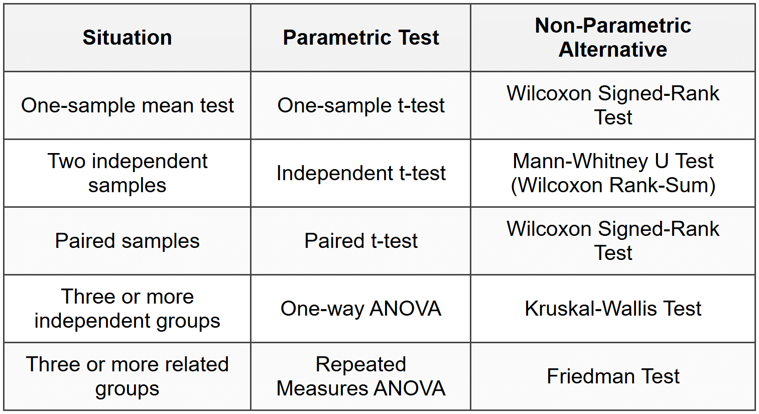
When to use non-parametric tests:

• Small sample size with non-normal data
• Ordinal data (ranks, ratings)
• Presence of extreme outliers
• Severe violations of parametric assumptions

Trade-off: Non-parametric tests are more robust but generally have lower statistical power than parametric tests when assumptions are met.

7. Effect Size

Effect Size measures the magnitude of difference or strength of relationship, independent of sample size.

7.1 Why Effect Size Matters

• Statistical vs Practical Significance: Small p-value doesn't mean large or important effect
• Sample size influence: Large samples can make trivial differences statistically significant
• Better interpretation: Effect size tells us "how much" difference exists, not just "is there a difference"

7.2 Common Effect Size Measures

7.2.1 Cohen's d

• Purpose: Standardized mean difference between two groups
• Formula: d = (x̄₁ - x̄₂) / s_pooled
• Interpretation: Small (d ≈ 0.2), Medium (d ≈ 0.5), Large (d ≈ 0.8)
• Use case: t-tests comparing two groups

7.2.2 Pearson's r

• Purpose: Measures strength of linear relationship
• Range: -1 to +1
• Interpretation: Small (|r| ≈ 0.1), Medium (|r| ≈ 0.3), Large (|r| ≈ 0.5)

7.2.3 Eta-squared (η²) and Omega-squared (ω²)

• Purpose: Proportion of variance explained in ANOVA
• Formula (η²): η² = SSB / SS_total
• Range: 0 to 1
• Interpretation: Small (η² ≈ 0.01), Medium (η² ≈ 0.06), Large (η² ≈ 0.14)
• ω² advantage: Less biased estimate than η² for population effect size

8. Confidence Intervals and Hypothesis Testing

8.1 Relationship Between CI and Hypothesis Testing

• Confidence Interval (CI): Range of plausible values for population parameter
• Connection to testing: If (1-α)×100% CI does not contain the null hypothesis value, reject H₀ at significance level α
• Example: 95% CI for difference in means [2.1, 5.8] excludes 0, so reject H₀: μ₁ = μ₂ at α = 0.05
• Advantage of CI: Provides both statistical significance AND range of plausible effect sizes

8.2 Two-sided vs One-sided Intervals

• Two-sided CI: Corresponds to two-tailed test
• One-sided CI: Corresponds to one-tailed test (upper or lower bound only)
• Best practice: Always report confidence intervals alongside p-values for complete interpretation

9. Multiple Testing Problem

9.1 The Problem

• Issue: Conducting multiple hypothesis tests increases overall Type I error rate
• Family-wise Error Rate (FWER): Probability of making at least one Type I error across all tests
• Example: 20 independent tests at α = 0.05 gives ~64% chance of at least one false positive
• Formula: FWER = 1 - (1 - α)^m, where m = number of tests

9.2 Corrections for Multiple Testing

9.2.1 Bonferroni Correction

• Method: Divide significance level by number of tests
• Adjusted α: α_adjusted = α / m
• Example: 10 tests with α = 0.05 requires α_adjusted = 0.005 for each test
• Limitation: Very conservative; reduces power substantially with many tests

9.2.2 False Discovery Rate (FDR)

• Method: Controls expected proportion of false positives among rejected hypotheses
• Less conservative: More powerful than Bonferroni for large number of tests
• Common procedure: Benjamini-Hochberg method
• Use case: Genomics, large-scale data mining, feature selection in ML

10. Practical Implementation Considerations

10.1 Sample Size Determination

• Factors affecting required n: Desired power, significance level, effect size, population variance
• Trade-off: Larger samples increase power but cost more in time and resources
• Power analysis: Calculate required sample size before data collection to ensure adequate power
• Post-hoc power: Calculating power after study is completed (generally discouraged)

10.2 Choosing the Right Test

Decision framework for selecting appropriate test:

1. Identify variable types: Continuous, categorical, ordinal?
2. Number of groups: One sample, two samples, multiple samples?
3. Sample relationship: Independent or paired/related?
4. Check assumptions: Normality, independence, equal variances?
5. Choose test: Parametric if assumptions met, non-parametric otherwise

10.3 Reporting Results

Essential components to report:

• Test used: Name and justify choice
• Descriptive statistics: Means, standard deviations, sample sizes for each group
• Test statistic value: t-value, z-value, F-value, χ² value, etc.
• Degrees of freedom: Where applicable
• p-value: Exact value (not just "p < 0.05")="" or="" report="" as="" p="">< 0.001="" for="" very="" small="">
• Effect size: Cohen's d, η², or other appropriate measure
• Confidence interval: For the parameter or difference being tested
• Conclusion: State decision clearly in context of problem

11. Common Mistakes and Misconceptions

11.1 Trap Alert: Common Errors

• Accepting H₀: Never say "accept null hypothesis"; only "fail to reject" or "insufficient evidence to reject"
• p-value misinterpretation: p-value is NOT probability that H₀ is true or that results are due to chance
• Confusing significance with importance: Statistically significant ≠ practically meaningful
• One vs two-tailed confusion: Two-tailed test requires evidence for difference in either direction; one-tailed is directional
• Ignoring assumptions: Applying tests without checking normality, independence, equal variance
• Sample size neglect: Large samples can make trivial differences significant; small samples lack power
• Post-hoc hypothesis: Formulating hypothesis after seeing data inflates Type I error
• p-hacking: Testing multiple hypotheses or models until finding significant result without correction
• Ignoring effect size: Reporting only p-values without magnitude of difference
• Wrong test for paired data: Using independent t-test when data is actually paired

11.2 Critical Thinking Guidelines

• Pre-registration: Define hypotheses and analysis plan before collecting data
• Assumption checking: Always verify test assumptions before interpreting results
• Contextual interpretation: Consider practical significance alongside statistical significance
• Replication: Single study results should be validated through replication
• Transparency: Report all tests conducted, not just significant ones

Hypothesis testing provides a rigorous framework for making data-driven decisions while quantifying uncertainty. By understanding the logic, assumptions, and proper interpretation of tests, you can confidently analyze data and draw valid conclusions. Always combine hypothesis testing with effect sizes, confidence intervals, and domain knowledge for comprehensive analysis. Remember that statistical significance is necessary but not sufficient-always consider the practical importance and context of your findings in business and data science applications.