Assignment : Pandas

Table of Contents
1. Section 1: Multiple Choice Questions
2. Section 2: Conceptual Questions
3. Section 3: Code Tracing / Output Prediction
4. Section 4: Coding Problems
5. Section 5: Challenge Problem (Optional)
6. Answer Key
View more

Section 1: Multiple Choice Questions

1. Q1. You have a DataFrame with missing values in multiple columns. You want to fill missing values in the 'Age' column with the median age, and missing values in the 'City' column with the string 'Unknown'. Which approach would be most appropriate?
   1. Use df.fillna() with a single value parameter
   2. Use df.fillna() with a dictionary mapping column names to fill values
   3. Use df.dropna() to remove all missing values first
   4. Use df.replace() with inplace=True for all columns
2. Q2. A DataFrame 'sales_data' contains columns 'Region', 'Product', and 'Revenue'. You need to find the total revenue for each combination of Region and Product. Which method would achieve this most efficiently?
   1. df.groupby('Region').sum()
   2. df.groupby(['Region', 'Product']).sum()
   3. df.pivot_table(values='Revenue', index='Region')
   4. df.sort_values(['Region', 'Product']).sum()
3. Q3. You have two DataFrames: 'employees' with columns ['emp_id', 'name', 'dept_id'] and 'departments' with columns ['dept_id', 'dept_name']. You want to create a result that includes all employees and their department names, keeping employees even if their department doesn't exist in the departments table. Which join type should you use?
   1. Inner join
   2. Right join
   3. Left join
   4. Outer join
4. Q4. You need to select all rows from a DataFrame where the 'Price' column is greater than 100 AND the 'Category' column equals 'Electronics'. Which syntax is correct?
   1. df[df['Price'] > 100 and df['Category'] == 'Electronics']
   2. df[(df['Price'] > 100) & (df['Category'] == 'Electronics')]
   3. df[df['Price'] > 100 | df['Category'] == 'Electronics']
   4. df.filter(Price > 100, Category == 'Electronics')
5. Q5. A time-series DataFrame has a datetime column that is currently stored as strings in the format 'YYYY-MM-DD'. Before performing time-based operations and setting it as the index, what should you do first?
   1. Directly set the string column as index using set_index()
   2. Convert the column to datetime using pd.to_datetime() then set as index
   3. Sort the DataFrame by the date column first
   4. Use df.astype('datetime') to convert the column

Section 2: Conceptual Questions

1. Q1. Explain the difference between a Pandas Series and a Pandas DataFrame. Provide an example scenario where you would use each data structure.
2. Q2. What is the purpose of the index in a Pandas DataFrame? Describe two advantages of having a meaningful index versus using the default integer index.
3. Q3. Describe the difference between loc and iloc indexing methods in Pandas. When would you choose one over the other?

Section 3: Code Tracing / Output Prediction

Code Snippet 1:

import pandas as pd data = {'Name': ['Alice', 'Bob', 'Charlie', 'David'], 'Score': [85, 90, 78, 92]} df = pd.DataFrame(data) result = df[df['Score'] > 80]['Name'].values print(result) print(type(result))

Predict the output of this code and explain what operations are being performed on the DataFrame.

Code Snippet 2:

import pandas as pd df = pd.DataFrame({ 'A': [1, 2, 3, 4], 'B': [10, 20, 30, 40], 'C': [100, 200, 300, 400] }) result1 = df.iloc[1:3, 0:2] result2 = df.loc[1:3, 'A':'B'] print("Result 1:") print(result1) print("\nResult 2:") print(result2)

Predict both outputs and explain why they are different or similar.

Section 4: Coding Problems

1. Q1. Create a DataFrame from scratch containing information about 5 books with columns: 'Title', 'Author', 'Year', and 'Price'. Then perform the following operations:
   • Display books published after 2015
   • Calculate the average price of all books
   • Sort the DataFrame by Year in descending order

   Sample Output Format:

   Books after 2015: Title Author Year Price ... Average Price: 25.50 Sorted by Year: Title Author Year Price ...

2. Q2. Write code to read a CSV file named 'students.csv' containing columns 'StudentID', 'Name', 'Math', 'Science', and 'English'. Then:
   • Add a new column 'Average' containing the average of Math, Science, and English scores
   • Find and display the student with the highest average
   • Filter and display students whose average is above 80

   Input format: Assume students.csv exists with appropriate data

   Expected operations: Read CSV, create calculated column, filter and display results

3. Q3. Given two DataFrames:
   • df1 with columns ['ProductID', 'ProductName', 'Category']
   • df2 with columns ['ProductID', 'QuantitySold', 'Revenue']
   Write code to merge these DataFrames on 'ProductID' and then group by 'Category' to find the total revenue for each category.

   Sample Input:

   df1: ProductID ProductName Category 0 101 Laptop Electronics 1 102 Mouse Electronics 2 103 Desk Furniture df2: ProductID QuantitySold Revenue 0 101 10 5000 1 102 50 500 2 103 5 1500

   Expected Output: Total revenue grouped by Category

4. Q4. Write a function that takes a DataFrame with a 'Date' column (as strings) and a 'Sales' column, then:
   • Converts the 'Date' column to datetime format
   • Sets 'Date' as the index
   • Resamples the data to monthly frequency and calculates the sum of sales for each month
   • Returns the resampled DataFrame

   Function signature:

   def resample_sales(df): # Your code here return resampled_df

   Sample Input: DataFrame with dates like '2023-01-15', '2023-01-20', '2023-02-10' and corresponding sales values

   Expected Output: Monthly aggregated sales data

Section 5: Challenge Problem (Optional)

You are given a DataFrame 'transactions' with columns: 'TransactionID', 'CustomerID', 'ProductID', 'Quantity', 'Price', and 'Date'. Write a comprehensive analysis script that:

1. Identifies the top 5 customers by total spending
2. Finds the most popular product (highest total quantity sold)
3. Calculates monthly revenue trends and identifies the month with highest revenue
4. Creates a pivot table showing total revenue by Customer and Product
5. Handles any missing values appropriately

Requirements:

• Use appropriate Pandas methods for grouping, aggregation, and pivoting
• Output should be well-formatted and clearly labeled
• Include comments explaining each major step
• The solution should be efficient and follow Pandas best practices

Bonus: Create a new column 'TotalAmount' (Quantity × Price) and use it in your calculations.

Answer Key

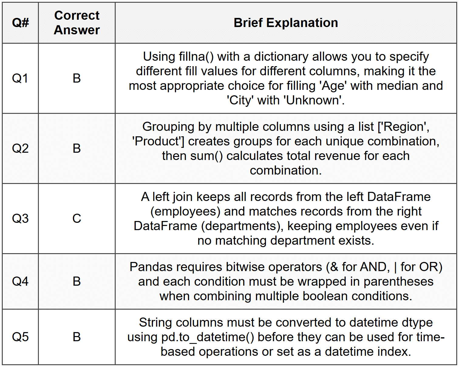
Section 1 - MCQ Answers

Section 2 Answers

Q1: A Pandas Series is a one-dimensional labeled array that can hold any data type, similar to a column in a spreadsheet or a single column from a database table. A DataFrame is a two-dimensional labeled data structure with columns that can be of different types, similar to a spreadsheet or SQL table. You would use a Series when working with a single variable or column of data, such as a list of temperatures or prices. You would use a DataFrame when working with multiple related variables, such as a dataset containing customer names, ages, purchases, and locations.

Q2: The index in a Pandas DataFrame serves as a label for each row, providing a way to identify and access specific rows of data. Two advantages of a meaningful index are: (1) It enables intuitive data access using loc indexing with meaningful labels rather than numeric positions, making code more readable and less prone to errors. (2) It facilitates efficient merging and joining operations, especially with time-series data where a datetime index allows for powerful time-based operations like resampling and time-based selection.

Q3: The loc method uses label-based indexing, meaning you access rows and columns using their actual labels (index names and column names). The iloc method uses integer position-based indexing, similar to how you would index a Python list or NumPy array. You would choose loc when you want to select data using meaningful labels or when working with non-integer indices like dates or names. You would choose iloc when you need to select data by position, such as getting the first three rows or every other row, regardless of what the actual index labels are.

Section 3 Answers

Code Snippet 1 Output:

['Alice' 'Bob' 'David'] <class 'numpy.ndarray'>

Explanation:
Step 1: df[df['Score'] > 80] filters the DataFrame to keep only rows where Score is greater than 80 (Alice: 85, Bob: 90, David: 92).
Step 2: ['Name'] selects only the Name column from the filtered DataFrame.
Step 3: .values converts the resulting Series to a NumPy array.
Step 4: The array contains the three names and the type is numpy.ndarray.

Code Snippet 2 Output:

Result 1: A B 1 2 20 2 3 30 Result 2: A B 1 2 20 2 3 30 3 4 40

Explanation:
Step 1: result1 uses iloc[1:3, 0:2] which uses integer position slicing. Row positions 1:3 means rows at index 1 and 2 (not including 3). Column positions 0:2 means columns 0 and 1 (A and B).
Step 2: result2 uses loc[1:3, 'A':'B'] which uses label-based slicing. Row labels 1:3 means index 1, 2, and 3 (inclusive on both ends). Column labels 'A':'B' means columns A and B.
Step 3: The key difference is that iloc uses exclusive end slicing while loc uses inclusive end slicing, so result2 includes row with index 3 while result1 does not.

Section 4 Answers

Q1 Solution:

import pandas as pd # Create DataFrame books_data = { 'Title': ['Python Basics', 'Data Science Guide', 'Machine Learning', 'Web Development', 'AI Fundamentals'], 'Author': ['John Smith', 'Jane Doe', 'Alice Brown', 'Bob Wilson', 'Carol White'], 'Year': [2014, 2018, 2020, 2016, 2021], 'Price': [29.99, 45.50, 55.00, 35.00, 49.99] } df = pd.DataFrame(books_data) # Display books published after 2015 print("Books after 2015:") books_after_2015 = df[df['Year'] > 2015] print(books_after_2015) # Calculate average price avg_price = df['Price'].mean() print(f"\nAverage Price: {avg_price:.2f}") # Sort by Year descending sorted_df = df.sort_values('Year', ascending=False) print("\nSorted by Year:") print(sorted_df)

Approach: Create a dictionary with book data, convert to DataFrame, use boolean indexing to filter, use mean() for average, and sort_values() with ascending=False for descending order.

Q2 Solution:

import pandas as pd # Read CSV file df = pd.read_csv('students.csv') # Add Average column df['Average'] = (df['Math'] + df['Science'] + df['English']) / 3 # Find student with highest average highest_avg_student = df.loc[df['Average'].idxmax()] print("Student with highest average:") print(highest_avg_student) # Filter students with average above 80 top_students = df[df['Average'] > 80] print("\nStudents with average above 80:") print(top_students)

Approach: Use read_csv() to load data, create a calculated column using arithmetic operations on multiple columns, use idxmax() to find the index of maximum value, and boolean indexing to filter students.

Q3 Solution:

import pandas as pd # Sample data creation df1 = pd.DataFrame({ 'ProductID': [101, 102, 103], 'ProductName': ['Laptop', 'Mouse', 'Desk'], 'Category': ['Electronics', 'Electronics', 'Furniture'] }) df2 = pd.DataFrame({ 'ProductID': [101, 102, 103], 'QuantitySold': [10, 50, 5], 'Revenue': [5000, 500, 1500] }) # Merge DataFrames merged_df = pd.merge(df1, df2, on='ProductID') # Group by Category and sum Revenue category_revenue = merged_df.groupby('Category')['Revenue'].sum() print("Total Revenue by Category:") print(category_revenue)

Approach: Use pd.merge() to join the DataFrames on ProductID, then use groupby() with sum() to aggregate revenue by category. The result shows total revenue for each category.

Q4 Solution:

import pandas as pd def resample_sales(df): # Convert Date column to datetime df['Date'] = pd.to_datetime(df['Date']) # Set Date as index df = df.set_index('Date') # Resample to monthly frequency and sum sales resampled_df = df['Sales'].resample('M').sum() # Convert back to DataFrame resampled_df = resampled_df.to_frame() return resampled_df # Example usage sample_data = pd.DataFrame({ 'Date': ['2023-01-15', '2023-01-20', '2023-02-10', '2023-02-25', '2023-03-05'], 'Sales': [1000, 1500, 2000, 1200, 1800] }) result = resample_sales(sample_data) print(result)

Approach: Convert the Date column to datetime using pd.to_datetime(), set it as index using set_index(), use resample('M') for monthly frequency with sum() aggregation, and convert the resulting Series back to a DataFrame for better readability.

Section 5 Answer

import pandas as pd # Assuming transactions DataFrame is already loaded # For demonstration, creating sample data transactions = pd.DataFrame({ 'TransactionID': range(1, 21), 'CustomerID': [1, 2, 1, 3, 2, 1, 4, 3, 2, 5, 1, 2, 3, 4, 5, 1, 2, 3, 4, 5], 'ProductID': [101, 102, 101, 103, 102, 103, 101, 102, 103, 101, 102, 101, 103, 102, 101, 103, 102, 101, 103, 102], 'Quantity': [2, 1, 3, 1, 2, 1, 4, 2, 1, 3, 1, 2, 1, 1, 2, 1, 3, 1, 2, 1], 'Price': [500, 300, 500, 200, 300, 200, 500, 300, 200, 500, 300, 500, 200, 300, 500, 200, 300, 500, 200, 300], 'Date': pd.date_range('2023-01-01', periods=20, freq='5D') }) # Handle missing values (if any) transactions = transactions.dropna() # Create TotalAmount column transactions['TotalAmount'] = transactions['Quantity'] * transactions['Price'] # 1. Top 5 customers by total spending customer_spending = transactions.groupby('CustomerID')['TotalAmount'].sum().sort_values(ascending=False).head(5) print("Top 5 Customers by Total Spending:") print(customer_spending) print("\n") # 2. Most popular product (highest total quantity sold) product_popularity = transactions.groupby('ProductID')['Quantity'].sum().sort_values(ascending=False) most_popular = product_popularity.index[0] total_qty = product_popularity.iloc[0] print(f"Most Popular Product: ProductID {most_popular} with {total_qty} units sold") print("\n") # 3. Monthly revenue trends transactions['YearMonth'] = transactions['Date'].dt.to_period('M') monthly_revenue = transactions.groupby('YearMonth')['TotalAmount'].sum() highest_month = monthly_revenue.idxmax() highest_revenue = monthly_revenue.max() print("Monthly Revenue Trends:") print(monthly_revenue) print(f"\nHighest Revenue Month: {highest_month} with ${highest_revenue}") print("\n") # 4. Pivot table: Total revenue by Customer and Product pivot = transactions.pivot_table( values='TotalAmount', index='CustomerID', columns='ProductID', aggfunc='sum', fill_value=0 ) print("Revenue by Customer and Product:") print(pivot)

Explanation: This comprehensive solution creates a TotalAmount column by multiplying Quantity and Price. It uses groupby() with sum() and sort_values() to find top customers, identifies the most popular product using total quantity, extracts year-month periods for monthly revenue analysis, and creates a pivot table to show the relationship between customers and products. The dropna() method handles missing values, and fill_value=0 in pivot_table ensures clean output for customer-product combinations with no transactions.