Signals And Systems

CHAPTER OVERVIEW

This chapter covers the fundamental principles of signals and systems as applied to electrical and computer engineering. Topics include classification of signals (continuous-time vs. discrete-time, periodic vs. aperiodic, energy vs. power), classification of systems (linear, time-invariant, causal, stable), time-domain and frequency-domain analysis, convolution, Fourier series and transforms, Laplace transforms, Z-transforms, transfer functions, frequency response, and sampling theory. Students will study mathematical representations of signals, system characterization through impulse and frequency responses, and analytical techniques for evaluating system behavior in both time and frequency domains. This chapter provides the theoretical foundation necessary for analyzing communication systems, control systems, digital signal processing, and filter design.

KEY CONCEPTS & THEORY

Signal Classification

Continuous-Time vs. Discrete-Time Signals

A continuous-time signal \( x(t) \) is defined for all values of time \( t \) in a continuous interval. A discrete-time signal \( x[n] \) is defined only at discrete time instants, typically at uniformly spaced intervals where \( n \) is an integer.

Periodic vs. Aperiodic Signals

A signal \( x(t) \) is periodic with period \( T \) if:

\[ x(t) = x(t + T) \text{ for all } t \]

The smallest positive value of \( T \) satisfying this condition is the fundamental period. The fundamental frequency is \( f_0 = 1/T \) Hz or \( \omega_0 = 2\pi/T \) rad/s. Signals that do not satisfy this condition are aperiodic.

Energy and Power Signals

The energy of a continuous-time signal over infinite time is:

\[ E = \int_{-\infty}^{\infty} |x(t)|^2 \, dt \]

The average power is:

\[ P = \lim_{T \to \infty} \frac{1}{2T} \int_{-T}^{T} |x(t)|^2 \, dt \]

A signal is an energy signal if \( 0 < e="">< \infty="" \)="" (which="" implies="" \(="" p="0" \)).="" a="" signal="" is="" a="">power signal if \( 0 < p="">< \infty="" \)="" (which="" implies="" \(="" e="\infty" \)).="" periodic="" signals="" are="" typically="" power="">

Even and Odd Signals

A signal \( x(t) \) is even if \( x(t) = x(-t) \) and odd if \( x(t) = -x(-t) \). Any signal can be decomposed into even and odd components:

\[ x_e(t) = \frac{x(t) + x(-t)}{2}, \quad x_o(t) = \frac{x(t) - x(-t)}{2} \]

System Classification

Linearity

A system is linear if it satisfies both additivity and homogeneity (scaling). For inputs \( x_1(t) \) and \( x_2(t) \) with outputs \( y_1(t) \) and \( y_2(t) \), and constants \( a \) and \( b \):

\[ a x_1(t) + b x_2(t) \rightarrow a y_1(t) + b y_2(t) \]

This is also known as the superposition property.

Time Invariance

A system is time-invariant if a time shift in the input causes an identical time shift in the output. If \( x(t) \rightarrow y(t) \), then \( x(t - t_0) \rightarrow y(t - t_0) \) for all \( t_0 \).

Causality

A system is causal if the output at any time depends only on present and past input values, not on future values. For a causal system, \( y(t_0) \) depends only on \( x(t) \) for \( t \leq t_0 \).

Stability

A system is bounded-input bounded-output (BIBO) stable if every bounded input produces a bounded output. For a linear time-invariant (LTI) system with impulse response \( h(t) \), the BIBO stability condition is:

\[ \int_{-\infty}^{\infty} |h(t)| \, dt < \infty="" \]="">

Convolution

Continuous-Time Convolution

For an LTI system with impulse response \( h(t) \) and input \( x(t) \), the output \( y(t) \) is given by the convolution integral:

\[ y(t) = x(t) * h(t) = \int_{-\infty}^{\infty} x(\tau) h(t - \tau) \, d\tau \]

Properties of convolution:

• Commutative: \( x(t) * h(t) = h(t) * x(t) \)
• Associative: \( [x(t) * h_1(t)] * h_2(t) = x(t) * [h_1(t) * h_2(t)] \)
• Distributive: \( x(t) * [h_1(t) + h_2(t)] = x(t) * h_1(t) + x(t) * h_2(t) \)

Discrete-Time Convolution

For discrete-time systems:

\[ y[n] = x[n] * h[n] = \sum_{k=-\infty}^{\infty} x[k] h[n-k] \]

Fourier Analysis

Fourier Series

A periodic continuous-time signal \( x(t) \) with period \( T \) can be represented as a Fourier series:

\[ x(t) = \sum_{k=-\infty}^{\infty} c_k e^{jk\omega_0 t} \]

where \( \omega_0 = 2\pi/T \) is the fundamental frequency and the Fourier series coefficients are:

\[ c_k = \frac{1}{T} \int_{T} x(t) e^{-jk\omega_0 t} \, dt \]

The trigonometric form is:

\[ x(t) = a_0 + \sum_{k=1}^{\infty} \left[ a_k \cos(k\omega_0 t) + b_k \sin(k\omega_0 t) \right] \]

where:

\[ a_0 = \frac{1}{T} \int_{T} x(t) \, dt, \quad a_k = \frac{2}{T} \int_{T} x(t) \cos(k\omega_0 t) \, dt, \quad b_k = \frac{2}{T} \int_{T} x(t) \sin(k\omega_0 t) \, dt \]

Fourier Transform

For aperiodic signals, the Fourier transform provides frequency-domain representation:

\[ X(j\omega) = \int_{-\infty}^{\infty} x(t) e^{-j\omega t} \, dt \]

The inverse Fourier transform is:

\[ x(t) = \frac{1}{2\pi} \int_{-\infty}^{\infty} X(j\omega) e^{j\omega t} \, d\omega \]

Important Fourier transform properties:

• Linearity: \( a x_1(t) + b x_2(t) \leftrightarrow a X_1(j\omega) + b X_2(j\omega) \)
• Time shifting: \( x(t - t_0) \leftrightarrow e^{-j\omega t_0} X(j\omega) \)
• Frequency shifting: \( e^{j\omega_0 t} x(t) \leftrightarrow X(j(\omega - \omega_0)) \)
• Time differentiation: \( \frac{dx(t)}{dt} \leftrightarrow j\omega X(j\omega) \)
• Convolution: \( x(t) * h(t) \leftrightarrow X(j\omega) H(j\omega) \)
• Multiplication: \( x(t) h(t) \leftrightarrow \frac{1}{2\pi} [X(j\omega) * H(j\omega)] \)
• Parseval's theorem: \( \int_{-\infty}^{\infty} |x(t)|^2 \, dt = \frac{1}{2\pi} \int_{-\infty}^{\infty} |X(j\omega)|^2 \, d\omega \)

Common Fourier Transform Pairs

• Impulse: \( \delta(t) \leftrightarrow 1 \)
• Constant: \( 1 \leftrightarrow 2\pi\delta(\omega) \)
• Rectangular pulse: \( \text{rect}(t/T) \leftrightarrow T \text{sinc}(\omega T/2) \)
• Exponential: \( e^{-at}u(t) \) (for \( a > 0 \)) \( \leftrightarrow \frac{1}{a + j\omega} \)
• Signum: \( \text{sgn}(t) \leftrightarrow \frac{2}{j\omega} \)

Laplace Transform

Definition and Properties

The Laplace transform generalizes the Fourier transform and is particularly useful for analyzing systems with initial conditions:

\[ X(s) = \int_{0^-}^{\infty} x(t) e^{-st} \, dt \]

where \( s = \sigma + j\omega \) is a complex variable. The inverse Laplace transform is:

\[ x(t) = \frac{1}{2\pi j} \int_{\sigma - j\infty}^{\sigma + j\infty} X(s) e^{st} \, ds \]

Key properties:

• Linearity: \( a x_1(t) + b x_2(t) \leftrightarrow a X_1(s) + b X_2(s) \)
• Time shifting: \( x(t - t_0)u(t - t_0) \leftrightarrow e^{-st_0} X(s) \)
• Differentiation: \( \frac{dx(t)}{dt} \leftrightarrow s X(s) - x(0^-) \)
• Integration: \( \int_{0^-}^{t} x(\tau) \, d\tau \leftrightarrow \frac{X(s)}{s} \)
• Convolution: \( x(t) * h(t) \leftrightarrow X(s) H(s) \)
• Initial value theorem: \( x(0^+) = \lim_{s \to \infty} s X(s) \)
• Final value theorem: \( \lim_{t \to \infty} x(t) = \lim_{s \to 0} s X(s) \) (if limit exists)

Common Laplace Transform Pairs

• Impulse: \( \delta(t) \leftrightarrow 1 \)
• Step: \( u(t) \leftrightarrow \frac{1}{s} \)
• Ramp: \( t u(t) \leftrightarrow \frac{1}{s^2} \)
• Exponential: \( e^{-at}u(t) \leftrightarrow \frac{1}{s + a} \)
• Sine: \( \sin(\omega_0 t)u(t) \leftrightarrow \frac{\omega_0}{s^2 + \omega_0^2} \)
• Cosine: \( \cos(\omega_0 t)u(t) \leftrightarrow \frac{s}{s^2 + \omega_0^2} \)

Transfer Functions and Frequency Response

Transfer Function

For an LTI system with zero initial conditions, the transfer function \( H(s) \) is the ratio of the Laplace transform of the output to the Laplace transform of the input:

\[ H(s) = \frac{Y(s)}{X(s)} \]

The transfer function is also the Laplace transform of the impulse response: \( H(s) = \mathcal{L}\{h(t)\} \).

Frequency Response

The frequency response \( H(j\omega) \) is obtained by substituting \( s = j\omega \) in the transfer function:

\[ H(j\omega) = |H(j\omega)| e^{j\angle H(j\omega)} \]

where \( |H(j\omega)| \) is the magnitude response and \( \angle H(j\omega) \) is the phase response. For a sinusoidal input \( x(t) = A\cos(\omega t + \phi) \), the steady-state output is:

\[ y_{ss}(t) = A|H(j\omega)|\cos(\omega t + \phi + \angle H(j\omega)) \]

Poles and Zeros

The transfer function can be expressed in factored form:

\[ H(s) = K \frac{(s - z_1)(s - z_2)\cdots(s - z_m)}{(s - p_1)(s - p_2)\cdots(s - p_n)} \]

where \( z_i \) are zeros and \( p_i \) are poles. For BIBO stability, all poles must have negative real parts (lie in the left half of the s-plane).

Z-Transform

Definition and Properties

The Z-transform is the discrete-time counterpart of the Laplace transform:

\[ X(z) = \sum_{n=-\infty}^{\infty} x[n] z^{-n} \]

where \( z \) is a complex variable. The inverse Z-transform recovers the discrete-time signal from \( X(z) \).

Key properties:

• Linearity: \( a x_1[n] + b x_2[n] \leftrightarrow a X_1(z) + b X_2(z) \)
• Time shifting: \( x[n - n_0] \leftrightarrow z^{-n_0} X(z) \)
• Convolution: \( x[n] * h[n] \leftrightarrow X(z) H(z) \)

Common Z-Transform Pairs

• Impulse: \( \delta[n] \leftrightarrow 1 \)
• Step: \( u[n] \leftrightarrow \frac{z}{z - 1} \), \( |z| > 1 \)
• Exponential: \( a^n u[n] \leftrightarrow \frac{z}{z - a} \), \( |z| > |a| \)
• Ramp: \( n u[n] \leftrightarrow \frac{z}{(z - 1)^2} \), \( |z| > 1 \)

Discrete-Time Transfer Function

For a discrete-time LTI system:

\[ H(z) = \frac{Y(z)}{X(z)} \]

The system is BIBO stable if all poles of \( H(z) \) lie inside the unit circle in the z-plane (i.e., \( |p_i| < 1="">

Sampling Theory

Sampling Theorem (Nyquist-Shannon)

A continuous-time signal \( x(t) \) with bandwidth \( B \) Hz (i.e., \( X(j\omega) = 0 \) for \( |\omega| > 2\pi B \)) can be perfectly reconstructed from its samples if the sampling frequency \( f_s \) satisfies:

\[ f_s \geq 2B \]

The minimum sampling rate \( f_s = 2B \) is called the Nyquist rate. If the sampling rate is below the Nyquist rate, aliasing occurs, causing distortion that cannot be corrected.

Sampling in the Frequency Domain

For a signal sampled at interval \( T_s = 1/f_s \), the spectrum of the sampled signal is periodic with period \( \omega_s = 2\pi f_s \):

\[ X_s(j\omega) = \frac{1}{T_s} \sum_{k=-\infty}^{\infty} X(j(\omega - k\omega_s)) \]

Filter Concepts

Ideal Filter Characteristics

• Lowpass filter: Passes frequencies below cutoff \( \omega_c \), blocks higher frequencies
• Highpass filter: Passes frequencies above cutoff \( \omega_c \), blocks lower frequencies
• Bandpass filter: Passes frequencies between \( \omega_1 \) and \( \omega_2 \), blocks others
• Bandstop (notch) filter: Blocks frequencies between \( \omega_1 \) and \( \omega_2 \), passes others

First-Order Systems

A first-order lowpass filter has transfer function:

\[ H(s) = \frac{K}{s + a} \]

The time constant is \( \tau = 1/a \), and the cutoff frequency (3-dB frequency) is \( \omega_c = a \) rad/s.

Second-Order Systems

A second-order system has the general form:

\[ H(s) = \frac{K\omega_n^2}{s^2 + 2\zeta\omega_n s + \omega_n^2} \]

where \( \omega_n \) is the natural frequency and \( \zeta \) is the damping ratio. System behavior depends on \( \zeta \):

• \( \zeta > 1 \): Overdamped
• \( \zeta = 1 \): Critically damped
• \( 0 < \zeta="">< 1="" \):="">
• \( \zeta = 0 \): Undamped

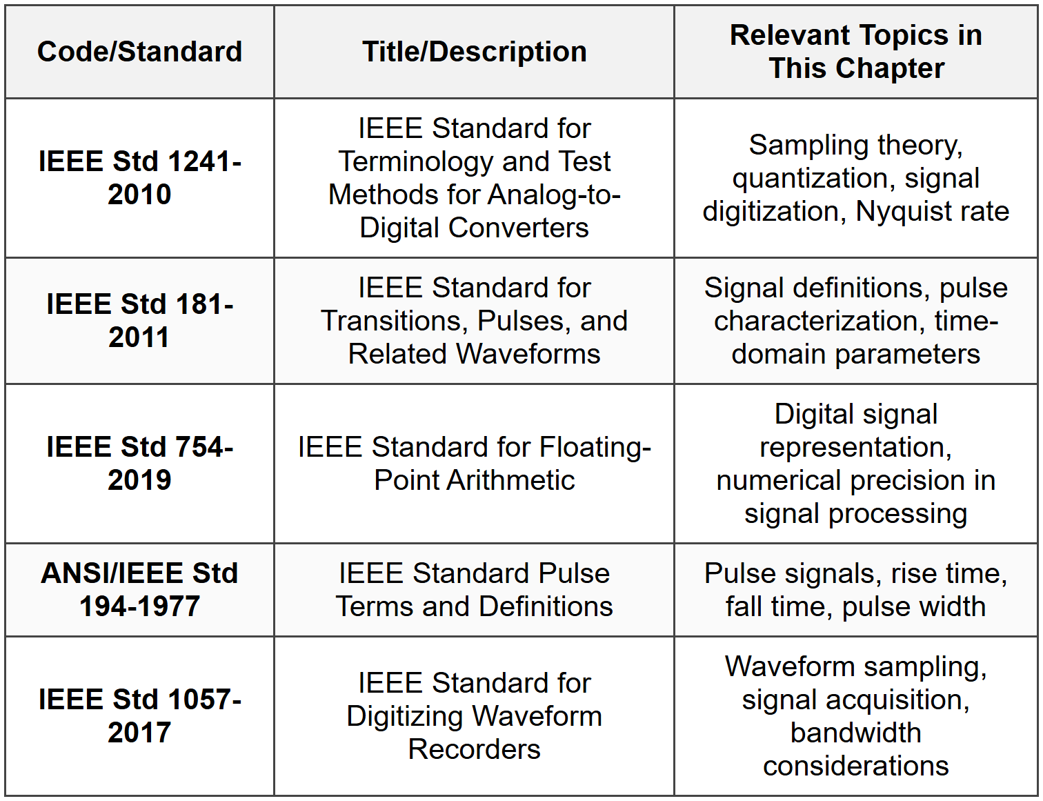
STANDARD CODES, STANDARDS & REFERENCES

SOLVED EXAMPLES

Example 1: Convolution and System Response

Problem Statement

An LTI system has an impulse response \( h(t) = e^{-2t}u(t) \), where \( u(t) \) is the unit step function. The input to the system is \( x(t) = e^{-t}u(t) \). Determine the output \( y(t) \) using convolution, and find the value of \( y(t) \) at \( t = 1 \) second.

Given Data

• Impulse response: \( h(t) = e^{-2t}u(t) \)
• Input signal: \( x(t) = e^{-t}u(t) \)
• Time of interest: \( t = 1 \) s

Find

Output \( y(t) \) and specifically \( y(1) \).

Solution

Step 1: Set up the convolution integral

The output is given by:

\[ y(t) = x(t) * h(t) = \int_{-\infty}^{\infty} x(\tau) h(t - \tau) \, d\tau \]

Step 2: Substitute the given functions

\[ y(t) = \int_{-\infty}^{\infty} e^{-\tau}u(\tau) \cdot e^{-2(t-\tau)}u(t-\tau) \, d\tau \]

Step 3: Determine integration limits

For the product \( u(\tau) \cdot u(t-\tau) \) to be non-zero:

• From \( u(\tau) \): \( \tau \geq 0 \)
• From \( u(t-\tau) \): \( \tau \leq t \)

Therefore, for \( t > 0 \), the limits are from 0 to \( t \):

\[ y(t) = \int_{0}^{t} e^{-\tau} \cdot e^{-2(t-\tau)} \, d\tau \]

Step 4: Simplify the integrand

\[ y(t) = \int_{0}^{t} e^{-\tau} \cdot e^{-2t+2\tau} \, d\tau = e^{-2t} \int_{0}^{t} e^{-\tau + 2\tau} \, d\tau = e^{-2t} \int_{0}^{t} e^{\tau} \, d\tau \]

Step 5: Evaluate the integral

\[ y(t) = e^{-2t} \left[ e^{\tau} \right]_{0}^{t} = e^{-2t} (e^{t} - e^{0}) = e^{-2t} (e^{t} - 1) \] \[ y(t) = e^{-t} - e^{-2t}, \quad t \geq 0 \]

Step 6: Calculate \( y(1) \)

\[ y(1) = e^{-1} - e^{-2} = 0.3679 - 0.1353 = 0.2326 \]

Answer

\( y(t) = (e^{-t} - e^{-2t})u(t) \) and \( y(1) = 0.233 \)

Example 2: Sampling and Aliasing

Problem Statement

A continuous-time signal consists of three sinusoidal components: \( x(t) = 2\cos(100\pi t) + 3\cos(300\pi t) + \cos(500\pi t) \). This signal is sampled at a rate of \( f_s = 400 \) Hz. Determine: (a) the highest frequency component in the signal, (b) the minimum sampling rate required to avoid aliasing, (c) whether aliasing occurs with the given sampling rate, and (d) if aliasing occurs, identify the apparent frequencies of the aliased components in the sampled signal.

Given Data

• Signal: \( x(t) = 2\cos(100\pi t) + 3\cos(300\pi t) + \cos(500\pi t) \)
• Sampling frequency: \( f_s = 400 \) Hz

Find

(a) Highest frequency component
(b) Minimum sampling rate (Nyquist rate)
(c) Whether aliasing occurs
(d) Apparent frequencies of aliased components

Solution

Step 1: Identify frequency components

For a cosine signal \( \cos(\omega t) \), the frequency is \( f = \omega/(2\pi) \) Hz.

First component: \( \omega_1 = 100\pi \) rad/s

\[ f_1 = \frac{100\pi}{2\pi} = 50 \text{ Hz} \]

Second component: \( \omega_2 = 300\pi \) rad/s

\[ f_2 = \frac{300\pi}{2\pi} = 150 \text{ Hz} \]

Third component: \( \omega_3 = 500\pi \) rad/s

\[ f_3 = \frac{500\pi}{2\pi} = 250 \text{ Hz} \]

Step 2: Determine highest frequency component (a)

\[ f_{\max} = 250 \text{ Hz} \]

Step 3: Calculate Nyquist rate (b)

According to the sampling theorem, the minimum sampling rate to avoid aliasing is:

\[ f_{s,\min} = 2f_{\max} = 2 \times 250 = 500 \text{ Hz} \]

Step 4: Check for aliasing (c)

Given sampling frequency: \( f_s = 400 \) Hz

Since \( f_s = 400 \text{ Hz} < f_{s,\min}="500" \text{="" hz}="" \),="" aliasing="" will="">

Step 5: Identify aliased frequencies (d)

For each frequency component \( f_i \), the apparent frequency after sampling can be found using:

\[ f_{\text{apparent}} = |f_i - k f_s| \]

where \( k \) is chosen such that \( f_{\text{apparent}} \) is in the range \( [0, f_s/2] \).

For \( f_1 = 50 \) Hz:

Since \( 50 < 200="" \)="" hz="" (which="" is="" \(="" f_s/2="" \)),="" no="" aliasing="">

\[ f_{1,\text{apparent}} = 50 \text{ Hz} \]

For \( f_2 = 150 \) Hz:

Since \( 150 < 200="" \)="" hz,="" no="" aliasing="">

\[ f_{2,\text{apparent}} = 150 \text{ Hz} \]

For \( f_3 = 250 \) Hz:

Since \( 250 > 200 \) Hz, aliasing occurs. We need to fold the frequency:

\[ f_{3,\text{apparent}} = f_s - f_3 = 400 - 250 = 150 \text{ Hz} \]

Step 6: Summary of apparent frequencies

The 50 Hz component appears at 50 Hz (no aliasing).
The 150 Hz component appears at 150 Hz (no aliasing).
The 250 Hz component appears at 150 Hz (aliased).

Note that the aliased 250 Hz component will be indistinguishable from the actual 150 Hz component, causing distortion.

Answer

(a) Highest frequency component: 250 Hz
(b) Minimum sampling rate (Nyquist rate): 500 Hz
(c) Yes, aliasing occurs because \( f_s = 400 \text{ Hz} < 500="" \text{="" hz}="">
(d) Apparent frequencies: 50 Hz (no aliasing), 150 Hz (no aliasing), 150 Hz (aliased from 250 Hz)

QUICK SUMMARY

PRACTICE QUESTIONS

Question 1: A discrete-time LTI system has impulse response \( h[n] = (0.5)^n u[n] \), where \( u[n] \) is the unit step sequence. The input to the system is \( x[n] = (0.25)^n u[n] \). Using Z-transform analysis, determine the transfer function \( H(z) \) and the output \( Y(z) \). What is the steady-state value of the output as \( n \to \infty \)?
(A) 0
(B) 1
(C) 0.5
(D) 2

Correct Answer: (A)

Explanation:

Step 1: Find \( H(z) \)
For \( h[n] = a^n u[n] \), the Z-transform is:
\( H(z) = \frac{z}{z - a} \) for \( |z| > |a| \)
Here \( a = 0.5 \), so:
\( H(z) = \frac{z}{z - 0.5} \)

Step 2: Find \( X(z) \)
For \( x[n] = (0.25)^n u[n] \):
\( X(z) = \frac{z}{z - 0.25} \) for \( |z| > 0.25 \)

Step 3: Calculate \( Y(z) \)
\( Y(z) = H(z) \cdot X(z) = \frac{z}{z - 0.5} \cdot \frac{z}{z - 0.25} = \frac{z^2}{(z - 0.5)(z - 0.25)} \)

Step 4: Apply final value theorem
The final value theorem for Z-transforms states:
\( \lim_{n \to \infty} y[n] = \lim_{z \to 1} (z - 1) Y(z) \)
This is valid if all poles of \( (z-1)Y(z) \) are inside the unit circle except for a possible simple pole at \( z = 1 \).

Step 5: Calculate limit
\( \lim_{z \to 1} (z - 1) \cdot \frac{z^2}{(z - 0.5)(z - 0.25)} = \lim_{z \to 1} \frac{(z-1)z^2}{(z - 0.5)(z - 0.25)} \)
\( = \frac{(1-1) \cdot 1^2}{(1 - 0.5)(1 - 0.25)} = \frac{0}{0.5 \times 0.75} = 0 \)

The steady-state value is 0. This makes physical sense because both the impulse response and input are decaying exponentials that approach zero as \( n \to \infty \).

─────────────────────────────────────────

Question 2: Which of the following statements regarding linear time-invariant (LTI) systems is TRUE?
(A) All causal systems are stable
(B) A system with impulse response \( h(t) = e^{2t}u(t) \) is BIBO stable
(C) The convolution of two causal signals always produces a causal signal
(D) All stable systems must be causal

Correct Answer: (C)

Explanation:

Option (A): False. Causality does not guarantee stability. A causal system can have an unbounded impulse response (e.g., \( h(t) = e^{2t}u(t) \)) and be unstable.

Option (B): False. For BIBO stability, we require \( \int_{-\infty}^{\infty} |h(t)| \, dt < \infty="">
For \( h(t) = e^{2t}u(t) \):
\( \int_{0}^{\infty} e^{2t} \, dt = \left[ \frac{e^{2t}}{2} \right]_{0}^{\infty} = \infty \)
The integral diverges, so the system is not BIBO stable.

Option (C): True. If \( x_1(t) = 0 \) for \( t < t_1="" \)="" and="" \(="" x_2(t)="0" \)="" for="" \(="" t="">< t_2="" \)="" (both="" causal="" from="" their="" respective="" starting="" times),="" then="" the="">
\( y(t) = \int_{-\infty}^{\infty} x_1(\tau) x_2(t - \tau) \, d\tau \)
The integrand is non-zero only when both \( \tau \geq t_1 \) and \( t - \tau \geq t_2 \), which implies \( \tau \geq t_1 \) and \( \tau \leq t - t_2 \).
For the integral to be non-zero, we need \( t_1 \leq t - t_2 \), or \( t \geq t_1 + t_2 \).
Thus \( y(t) = 0 \) for \( t < t_1="" +="" t_2="" \),="" making="" it="" causal="" from="" time="" \(="" t_1="" +="" t_2="">

Option (D): False. Stability and causality are independent properties. A stable system need not be causal (e.g., \( h(t) = e^{-|t|} \) is stable but non-causal).

─────────────────────────────────────────

Question 3: An engineer is designing a digital audio recording system for a music studio. The system must accurately capture instruments with frequency content up to 18 kHz. The anti-aliasing filter has a transition band from 18 kHz to 22 kHz. To ensure compliance with the Nyquist criterion and provide adequate margin for practical filter implementation, what is the minimum acceptable sampling rate for this system?
(A) 36 kHz
(B) 40 kHz
(C) 44 kHz
(D) 48 kHz

Correct Answer: (C)

Explanation:

Step 1: Identify maximum signal frequency
The maximum frequency content to be captured is \( f_{\max} = 18 \) kHz.

Step 2: Calculate Nyquist rate
The theoretical Nyquist rate is:
\( f_{s,min} = 2 f_{\max} = 2 \times 18 = 36 \text{ kHz} \)

Step 3: Consider practical filter constraints
The anti-aliasing filter has a transition band from 18 kHz to 22 kHz. This means the filter begins to attenuate at 18 kHz and should provide sufficient attenuation by 22 kHz to prevent aliasing.

For adequate anti-aliasing protection, the sampling frequency must be high enough that the first image (which appears at \( f_s - f \)) does not overlap with the signal band after accounting for the filter's transition band.

The filter stops passing signals effectively at approximately 22 kHz (upper edge of transition band). To prevent aliasing, we need:
\( f_s - f_{\max} \geq 22 \text{ kHz} - f_{\max} \)
Or more practically: \( f_s \geq 2 \times 22 = 44 \text{ kHz} \)

Step 4: Compare with standard sampling rates
Option (A) 36 kHz: This equals the theoretical Nyquist rate but provides no guard band for the filter transition region.
Option (B) 40 kHz: This provides some margin but may be insufficient for the specified transition band.
Option (C) 44 kHz: This is the standard CD audio sampling rate (44.1 kHz typically), providing adequate margin.
Option (D) 48 kHz: While this would work, it exceeds the minimum requirement.

Given that the transition band extends to 22 kHz, the minimum sampling rate should be at least 44 kHz to ensure that frequencies above 22 kHz (which are attenuated by the filter) do not alias back into the passband below 18 kHz.

─────────────────────────────────────────

Question 4: According to IEEE Std 1241-2010 (Standard for Terminology and Test Methods for Analog-to-Digital Converters), the effective number of bits (ENOB) is a measure of ADC performance that accounts for all sources of error. If an analog-to-digital converter (ADC) has a signal-to-noise and distortion ratio (SINAD) of 68 dB, what is the effective number of bits (ENOB) for this ADC? The relationship is given by: ENOB = (SINAD - 1.76) / 6.02.
(A) 9.5 bits
(B) 10.0 bits
(C) 11.0 bits
(D) 11.5 bits

Correct Answer: (C)

Explanation:

Step 1: Identify given parameters
SINAD = 68 dB
Formula: ENOB = (SINAD - 1.76) / 6.02

Step 2: Apply the formula
\( \text{ENOB} = \frac{68 - 1.76}{6.02} = \frac{66.24}{6.02} = 11.00 \text{ bits} \)

Step 3: Interpretation
The effective number of bits represents the actual resolution of the ADC after accounting for noise, distortion, and other non-idealities. According to IEEE Std 1241-2010, this metric provides a more realistic assessment of ADC performance than the nominal bit count.

The formula is derived from the relationship between the ideal signal-to-noise ratio for an N-bit ADC:
\( \text{SNR}_{\text{ideal}} = 6.02N + 1.76 \text{ dB} \)

For SINAD = 68 dB, the effective number of bits is 11.0 bits.

─────────────────────────────────────────

Question 5: The frequency response data for an LTI system is provided in the table below. Based on this data, determine the approximate 3-dB bandwidth of the system and classify the filter type.

(A) 3 kHz, lowpass filter
(B) 4 kHz, bandpass filter
(C) 3 kHz, highpass filter
(D) 5 kHz, lowpass filter

Correct Answer: (A)

Explanation:

Step 1: Define 3-dB bandwidth
The 3-dB bandwidth is the frequency at which the magnitude response drops to -3 dB relative to the DC (maximum) value, or equivalently where \( |H(j\omega)| = 0.707 \times |H(0)| \) in linear units.

Step 2: Identify DC gain
At \( f = 0 \) Hz: \( |H(0)| = 1.00 \) (0 dB)

Step 3: Find 3-dB point
We need to find where the magnitude is approximately -3 dB or \( |H(j\omega)| \approx 0.707 \).

From the table:
At 2000 Hz: -1.41 dB (above -3 dB)
At 3000 Hz: -2.97 dB (approximately -3 dB)
At 4000 Hz: -5.19 dB (below -3 dB)

The magnitude at 3000 Hz is -2.97 dB, which is very close to -3 dB. The corresponding linear magnitude is 0.71, which is approximately 0.707.

Step 4: Classify filter type
Examining the data:
- Maximum gain occurs at 0 Hz (DC)
- Magnitude decreases monotonically as frequency increases
- No indication of a lower cutoff frequency

This behavior is characteristic of a lowpass filter.

Step 5: Conclusion
The 3-dB bandwidth is approximately 3 kHz, and the system is a lowpass filter.