Formula Sheet: Process Control

Transfer Functions and Block Diagrams

Laplace Transform Basics

Definition:

\[F(s) = \mathcal{L}\{f(t)\} = \int_0^\infty f(t)e^{-st}dt\]

Variables:

• s = complex frequency variable (rad/s or s^-1)
• f(t) = time-domain function
• F(s) = Laplace transform of f(t)

Common Laplace Transforms:

• Unit step: \(\mathcal{L}\{1\} = \frac{1}{s}\)
• Ramp: \(\mathcal{L}\{t\} = \frac{1}{s^2}\)
• Exponential: \(\mathcal{L}\{e^{-at}\} = \frac{1}{s+a}\)
• Sine: \(\mathcal{L}\{\sin(\omega t)\} = \frac{\omega}{s^2 + \omega^2}\)
• Cosine: \(\mathcal{L}\{\cos(\omega t)\} = \frac{s}{s^2 + \omega^2}\)
• Derivative: \(\mathcal{L}\left\{\frac{df}{dt}\right\} = sF(s) - f(0)\)
• Integral: \(\mathcal{L}\left\{\int_0^t f(\tau)d\tau\right\} = \frac{F(s)}{s}\)

Transfer Function Definition

\[G(s) = \frac{Y(s)}{U(s)}\]

Variables:

• G(s) = transfer function
• Y(s) = Laplace transform of output variable
• U(s) = Laplace transform of input variable
• Assumes zero initial conditions

Block Diagram Algebra

Series (Cascade):

\[G_{total} = G_1 \times G_2 \times G_3 \times ... \times G_n\]

Parallel:

\[G_{total} = G_1 + G_2 + G_3 + ... + G_n\]

Feedback Loop (Negative Feedback):

\[G_{closed} = \frac{G}{1 + GH}\]

• G = forward path transfer function
• H = feedback path transfer function

Feedback Loop (Positive Feedback):

\[G_{closed} = \frac{G}{1 - GH}\]

Deviation Variables

\[y'(t) = y(t) - y_s\] \[u'(t) = u(t) - u_s\]

Variables:

• y'(t) = output deviation variable
• u'(t) = input deviation variable
• y_s = steady-state output value
• u_s = steady-state input value

First-Order Systems

Standard First-Order Transfer Function

\[G(s) = \frac{K}{\tau s + 1}\]

Variables:

• K = process gain (dimensionless or with appropriate units)
• τ = time constant (time units, typically seconds or minutes)
• s = Laplace variable

Step Response of First-Order System

\[y(t) = K A \left(1 - e^{-t/\tau}\right)\]

Variables:

• y(t) = output response
• A = magnitude of step input
• K = process gain
• τ = time constant

Key Time Response Characteristics:

• At t = τ: y(τ) = 0.632 KA (63.2% of final value)
• At t = 2τ: y = 0.865 KA (86.5% of final value)
• At t = 3τ: y = 0.950 KA (95.0% of final value)
• At t = 4τ: y = 0.982 KA (98.2% of final value)
• At t = 5τ: y = 0.993 KA (99.3% of final value, essentially settled)

First-Order with Time Delay

\[G(s) = \frac{K e^{-\theta s}}{\tau s + 1}\]

Variables:

• θ = time delay or dead time (same units as τ)
• e^-θs = dead time element

Step Response:

\[y(t) = \begin{cases} 0 & t < \theta="" \\="" k="" a="" \left(1="" -="" e^{-(t-\theta)/\tau}\right)="" &="" t="" \geq="" \theta="" \end{cases}\]="">

Second-Order Systems

Standard Second-Order Transfer Function

\[G(s) = \frac{K\omega_n^2}{s^2 + 2\zeta\omega_n s + \omega_n^2}\]

Alternative Form:

\[G(s) = \frac{K}{\tau^2 s^2 + 2\zeta\tau s + 1}\]

Variables:

• K = steady-state gain
• ω_n = natural frequency (rad/time)
• ζ = damping ratio (dimensionless)
• τ = time constant where τ = 1/ω_n

Damping Categories

• Overdamped: ζ > 1 (two real, distinct poles)
• Critically damped: ζ = 1 (two real, equal poles)
• Underdamped: 0 < ζ="">< 1="" (complex="" conjugate="">
• Undamped: ζ = 0 (purely imaginary poles)

Underdamped Step Response

\[y(t) = K A \left[1 - \frac{e^{-\zeta\omega_n t}}{\sqrt{1-\zeta^2}}\sin\left(\omega_d t + \phi\right)\right]\]

Where:

\[\omega_d = \omega_n\sqrt{1-\zeta^2}\] \[\phi = \cos^{-1}(\zeta) = \tan^{-1}\left(\frac{\sqrt{1-\zeta^2}}{\zeta}\right)\]

Variables:

• ω_d = damped natural frequency (rad/time)
• φ = phase angle (radians)

Performance Characteristics (Underdamped)

Percent Overshoot:

\[OS\% = 100 \times e^{-\pi\zeta/\sqrt{1-\zeta^2}}\]

Rise Time (0% to 100%):

\[t_r = \frac{\pi - \phi}{\omega_d}\]

Peak Time:

\[t_p = \frac{\pi}{\omega_d} = \frac{\pi}{\omega_n\sqrt{1-\zeta^2}}\]

Settling Time (2% criterion):

\[t_s = \frac{4}{\zeta\omega_n}\]

Settling Time (5% criterion):

\[t_s = \frac{3}{\zeta\omega_n}\]

Decay Ratio:

\[DR = e^{-2\pi\zeta/\sqrt{1-\zeta^2}} = (OS\%)^2\]

Controller Types and Equations

Proportional (P) Controller

Time Domain:

\[u(t) = K_c e(t) + \bar{u}\]

Deviation Form:

\[u'(t) = K_c e(t)\]

Transfer Function:

\[G_c(s) = K_c\]

Variables:

• u(t) = controller output (manipulated variable)
• e(t) = error = y_sp - y (setpoint - measurement)
• K_c = controller gain (dimensionless or %-to-% typically)
• ū = bias or steady-state output

Proportional-Integral (PI) Controller

Time Domain:

\[u(t) = K_c\left[e(t) + \frac{1}{\tau_I}\int_0^t e(t')dt'\right] + \bar{u}\]

Transfer Function:

\[G_c(s) = K_c\left(1 + \frac{1}{\tau_I s}\right) = K_c\frac{\tau_I s + 1}{\tau_I s}\]

Alternative Form (using reset rate):

\[G_c(s) = K_c\left(1 + \frac{K_I}{s}\right)\]

Variables:

• τ_I = integral time or reset time (time units)
• K_I = integral gain = 1/τ_I (1/time)

Proportional-Derivative (PD) Controller

Time Domain:

\[u(t) = K_c\left[e(t) + \tau_D\frac{de(t)}{dt}\right] + \bar{u}\]

Transfer Function (Ideal):

\[G_c(s) = K_c(1 + \tau_D s)\]

Transfer Function (Real/Practical with Filter):

\[G_c(s) = K_c\left(1 + \frac{\tau_D s}{\alpha\tau_D s + 1}\right)\]

Variables:

• τ_D = derivative time (time units)
• α = derivative filter constant (typically 0.05 to 0.2)

Proportional-Integral-Derivative (PID) Controller

Time Domain (Ideal):

\[u(t) = K_c\left[e(t) + \frac{1}{\tau_I}\int_0^t e(t')dt' + \tau_D\frac{de(t)}{dt}\right] + \bar{u}\]

Transfer Function (Ideal):

\[G_c(s) = K_c\left(1 + \frac{1}{\tau_I s} + \tau_D s\right)\]

Transfer Function (Series/Interacting Form):

\[G_c(s) = K_c'\left(1 + \frac{1}{\tau_I' s}\right)(1 + \tau_D' s)\]

Transfer Function (Parallel Form):

\[G_c(s) = K_p + \frac{K_I}{s} + K_D s\]

Relationships:

• K_p = K_c
• K_I = K_c/τ_I
• K_D = K_cτ_D

Controller Action: Direct vs. Reverse

Direct (Positive) Action:

• Controller output increases when measurement increases
• e = y_sp - y

Reverse (Negative) Action:

• Controller output decreases when measurement increases
• e = y - y_sp or use negative K_c

Closed-Loop Control System Analysis

Standard Feedback Control Loop

Closed-Loop Transfer Function (Servo Response):

\[\frac{Y(s)}{Y_{sp}(s)} = \frac{G_c G_v G_p G_m}{1 + G_c G_v G_p G_m}\]

Disturbance Response (Regulatory Response):

\[\frac{Y(s)}{D(s)} = \frac{G_d}{1 + G_c G_v G_p G_m}\]

Variables:

• G_c = controller transfer function
• G_v = final control element (valve) transfer function
• G_p = process transfer function
• G_m = measurement/sensor transfer function
• G_d = disturbance transfer function
• Y_sp = setpoint
• D = disturbance

Open-Loop Transfer Function

\[G_{OL}(s) = G_c G_v G_p G_m\]

Note: Often G_v and G_m are assumed to be 1 (unity) for simplicity.

Characteristic Equation

\[1 + G_{OL}(s) = 0\]

The roots of this equation are the closed-loop poles which determine stability.

Offset (Steady-State Error)

Final Value Theorem:

\[e_{ss} = \lim_{t \to \infty} e(t) = \lim_{s \to 0} s E(s)\]

For P-only Control with Unit Step Setpoint Change:

\[e_{ss} = \frac{1}{1 + K_c K_p}\]

Variables:

• e_ss = steady-state error (offset)
• K_p = process steady-state gain

Note: PI and PID controllers eliminate offset for step changes in setpoint or load (integral action).

Stability Analysis

Routh-Hurwitz Stability Criterion

General Characteristic Equation:

\[a_n s^n + a_{n-1} s^{n-1} + ... + a_1 s + a_0 = 0\]

Routh Array Construction:

• First row: a_n, a_n-2, a_n-4, ...
• Second row: a_n-1, a_n-3, a_n-5, ...
• Subsequent rows calculated using determinant formula

Stability Criterion:

• System is stable if all elements in the first column of the Routh array have the same sign (positive)
• Number of sign changes in first column = number of roots with positive real parts

Bode Stability Criterion

Gain Margin (GM):

\[GM = \frac{1}{|G_{OL}(j\omega_{pc})|}\] \[GM_{dB} = -20\log_{10}|G_{OL}(j\omega_{pc})|\]

Phase Margin (PM):

\[PM = 180° + \angle G_{OL}(j\omega_{gc})\]

Variables:

• ω_pc = phase crossover frequency (where phase = -180°)
• ω_gc = gain crossover frequency (where |G_OL| = 1 or 0 dB)

Stability Conditions:

• For stability: GM > 1 (or GM_dB > 0) and PM > 0°
• Typical design targets: GM > 1.7 (5 dB), PM > 30° to 45°

Ultimate Gain and Period

Ultimate Gain (K_u):

• Controller gain at which system becomes marginally stable (sustained oscillations)
• Related to gain margin: K_u = K_c × GM

Ultimate Period (P_u):

\[P_u = \frac{2\pi}{\omega_{pc}}\]

• P_u = period of sustained oscillations at K_u
• ω_pc = frequency at which phase angle = -180°

Controller Tuning Methods

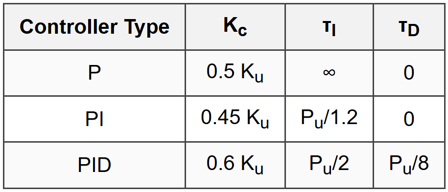
Ziegler-Nichols Closed-Loop (Ultimate Gain) Method

Procedure:

• Use P-only control, increase K_c until sustained oscillations occur
• Record ultimate gain K_u and ultimate period P_u

Tuning Parameters:

Ziegler-Nichols Open-Loop (Process Reaction Curve) Method

Procedure:

• Apply step change to process in open loop
• Draw tangent line at maximum slope of response curve
• Determine dead time θ and time constant τ from tangent intercepts
• Calculate R = ΔY/(Δu × τ) where ΔY/Δu is normalized process gain

Tuning Parameters:

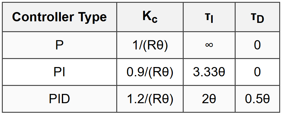
Variables:

• R = reaction rate = slope at inflection point / (process gain)
• θ = apparent dead time (time units)
• τ = apparent time constant (time units)

Cohen-Coon Tuning Method

Based on same process parameters as Z-N open-loop (θ, τ, K_p):

\[\tau_0 = \frac{\theta}{\tau}\]

Tuning Parameters:

P Controller:

\[K_c = \frac{\tau}{K_p\theta}\left(1 + \frac{\tau_0}{3}\right)\]

PI Controller:

\[K_c = \frac{\tau}{K_p\theta}\left(0.9 + \frac{\tau_0}{12}\right)\] \[\tau_I = \theta\frac{30 + 3\tau_0}{9 + 20\tau_0}\]

PID Controller:

\[K_c = \frac{\tau}{K_p\theta}\left(\frac{4}{3} + \frac{\tau_0}{4}\right)\] \[\tau_I = \theta\frac{32 + 6\tau_0}{13 + 8\tau_0}\] \[\tau_D = \theta\frac{4}{11 + 2\tau_0}\]

ITAE (Integral of Time-Weighted Absolute Error) Tuning

For First-Order Plus Dead Time (FOPDT) Process:

PI Controller (Disturbance Rejection):

\[K_c = \frac{0.859}{K_p}\left(\frac{\theta}{\tau}\right)^{-0.977}\] \[\tau_I = \frac{\tau}{0.674}\left(\frac{\theta}{\tau}\right)^{-0.680}\]

PID Controller (Disturbance Rejection):

\[K_c = \frac{1.357}{K_p}\left(\frac{\theta}{\tau}\right)^{-0.947}\] \[\tau_I = \frac{\tau}{0.842}\left(\frac{\theta}{\tau}\right)^{-0.738}\] \[\tau_D = 0.381\tau\left(\frac{\theta}{\tau}\right)^{0.995}\]

IMC (Internal Model Control) Tuning

For FOPDT Process:

PI Controller:

\[K_c = \frac{\tau}{K_p(\lambda + \theta)}\] \[\tau_I = \tau\]

PID Controller:

\[K_c = \frac{\tau}{K_p\lambda}\] \[\tau_I = \tau\] \[\tau_D = 0\]

Variables:

• λ = IMC filter time constant (tuning parameter, typically λ = θ to 2θ)
• Smaller λ gives faster, more aggressive control
• Larger λ gives slower, more conservative control

Frequency Response

Frequency Response Function

\[G(j\omega) = |G(j\omega)|e^{j\phi(\omega)}\]

Magnitude:

\[|G(j\omega)| = \sqrt{[\text{Re}(G(j\omega))]^2 + [\text{Im}(G(j\omega))]^2}\]

Phase Angle:

\[\phi(\omega) = \tan^{-1}\left(\frac{\text{Im}(G(j\omega))}{\text{Re}(G(j\omega))}\right)\]

In Decibels:

\[|G(j\omega)|_{dB} = 20\log_{10}|G(j\omega)|\]

First-Order System Frequency Response

\[G(j\omega) = \frac{K}{j\omega\tau + 1}\]

Magnitude:

\[|G(j\omega)| = \frac{K}{\sqrt{1 + (\omega\tau)^2}}\]

Phase:

\[\phi(\omega) = -\tan^{-1}(\omega\tau)\]

At Corner Frequency (ω = 1/τ):

• |G(jω)| = K/√2 = 0.707K
• |G(jω)|_dB = -3 dB (relative to K)
• φ = -45°

Second-Order System Frequency Response

\[G(j\omega) = \frac{K\omega_n^2}{-\omega^2 + 2j\zeta\omega_n\omega + \omega_n^2}\]

Magnitude:

\[|G(j\omega)| = \frac{K\omega_n^2}{\sqrt{(\omega_n^2 - \omega^2)^2 + (2\zeta\omega_n\omega)^2}}\]

Phase:

\[\phi(\omega) = -\tan^{-1}\left(\frac{2\zeta\omega_n\omega}{\omega_n^2 - \omega^2}\right)\]

Resonant Peak (for ζ <>

\[M_r = \frac{K}{2\zeta\sqrt{1-\zeta^2}}\]

Resonant Frequency:

\[\omega_r = \omega_n\sqrt{1 - 2\zeta^2}\]

Bode Plot Asymptotes

Gain (K):

• Magnitude: 20log₁₀K (constant horizontal line)
• Phase: 0°

Integrator (1/s):

• Slope: -20 dB/decade
• Phase: -90° (constant)

Differentiator (s):

• Slope: +20 dB/decade
• Phase: +90° (constant)

First-Order Lag (1/(τs + 1)):

• Low frequency (ω < 1/τ):="" 0="">
• High frequency (ω >> 1/τ): -20 dB/decade
• Corner frequency: ω = 1/τ
• Phase: 0° to -90°

First-Order Lead (τs + 1):

• Low frequency: 0 dB/decade
• High frequency: +20 dB/decade
• Corner frequency: ω = 1/τ
• Phase: 0° to +90°

Second-Order System:

• Low frequency: 0 dB/decade
• High frequency: -40 dB/decade
• Corner frequency: ω = ω_n
• Phase: 0° to -180°

Dead Time (e^-θs):

• Magnitude: |G(jω)| = 1 (0 dB) for all frequencies
• Phase: φ(ω) = -θω (radians), linear decrease with frequency

Advanced Control Strategies

Cascade Control

Structure:

• Primary (master) controller output becomes setpoint for secondary (slave) controller
• Inner loop responds faster than outer loop

Overall Transfer Function:

\[\frac{Y_1(s)}{Y_{sp,1}(s)} = \frac{G_{c1}G_{c2}G_{p1}G_{p2}}{1 + G_{c2}G_{p2} + G_{c1}G_{c2}G_{p1}G_{p2}}\]

Variables:

• G_c1 = primary controller
• G_c2 = secondary controller
• G_p1 = primary process
• G_p2 = secondary process

Design Guidelines:

• Tune secondary loop first (with primary on manual)
• Then tune primary loop
• Secondary loop should be 3-10 times faster than primary

Feedforward Control

Ideal Feedforward Controller:

\[G_{FF}(s) = -\frac{G_d(s)}{G_p(s)}\]

Variables:

• G_FF = feedforward controller transfer function
• G_d = disturbance-to-output transfer function
• G_p = manipulated variable-to-output transfer function

Combined Feedforward-Feedback Output:

\[u(t) = u_{FF}(t) + u_{FB}(t)\]

Lead-Lag Feedforward Controller:

\[G_{FF}(s) = K_{FF}\frac{\tau_1 s + 1}{\tau_2 s + 1}\]

Ratio Control

Flow Ratio:

\[R = \frac{F_B}{F_A}\]

Controller Output:

\[F_{B,sp} = R \times F_A\]

Variables:

• F_A = wild (uncontrolled) flow rate
• F_B = controlled flow rate
• R = desired ratio

Split-Range Control

One controller output signal operates two or more final control elements over different ranges:

• Valve 1 operates: 0-50% controller output
• Valve 2 operates: 50-100% controller output

Override (Selective) Control

Low Select:

\[u = \min(u_1, u_2, ..., u_n)\]

High Select:

\[u = \max(u_1, u_2, ..., u_n)\]

Used for constraint control and safety limits.

Decoupling Control (Multivariable Systems)

For 2×2 System:

\[Y_1(s) = G_{11}(s)U_1(s) + G_{12}(s)U_2(s)\] \[Y_2(s) = G_{21}(s)U_1(s) + G_{22}(s)U_2(s)\]

Ideal Decoupler:

\[D_{12}(s) = -\frac{G_{12}(s)}{G_{11}(s)}\] \[D_{21}(s) = -\frac{G_{21}(s)}{G_{22}(s)}\]

Variables:

• G_ij = transfer function from input j to output i
• D_ij = decoupler from loop j to loop i

Control Valve Characteristics

Valve Sizing Equation

Liquid Flow (Incompressible):

\[Q = C_v\sqrt{\frac{\Delta P}{SG}}\]

Variables:

• Q = flow rate (gpm for US units)
• C_v = valve flow coefficient (gpm/psi^0.5)
• ΔP = pressure drop across valve (psi)
• SG = specific gravity (dimensionless, water = 1.0)

Gas Flow (for ΔP/P₁ <>

\[Q = C_v\sqrt{\frac{1360 \Delta P P_1}{SG_g T}}\]

Variables:

• Q = flow rate (scfh, standard ft³/hr)
• P₁ = upstream pressure (psia)
• SG_g = gas specific gravity (air = 1.0)
• T = absolute temperature (°R = °F + 460)

Valve Characteristics

Linear:

\[F = x\]

• Flow proportional to valve position

Equal Percentage:

\[F = R^{x-1}\]

• R = rangeability (typically 20-50)
• x = fraction of valve opening (0 to 1)
• Equal percentage change in flow per equal percentage change in valve position

Quick Opening:

\[F = \sqrt{x}\]

• Maximum change near closed position

Installed Valve Gain

\[K_v = \frac{dQ}{dx}\]

At Operating Point:

\[K_v = \frac{Q_{max} - Q_{min}}{x_{max} - x_{min}}\]

Variables:

• K_v = valve gain
• Q = flow rate
• x = valve position (typically % open)

Sensor and Transmitter Dynamics

First-Order Sensor

\[G_m(s) = \frac{K_m}{\tau_m s + 1}\]

Variables:

• K_m = measurement gain (typically 1 for 4-20 mA signal)
• τ_m = sensor time constant

Thermocouple/RTD Time Constant

\[\tau_s = \frac{mc_p}{hA}\]

Variables:

• m = mass of sensor element
• c_p = specific heat of sensor
• h = heat transfer coefficient
• A = surface area of sensor

Transmitter Span and Zero

Output Signal:

\[I = I_{min} + \frac{I_{max} - I_{min}}{PV_{max} - PV_{min}}(PV - PV_{min})\]

For 4-20 mA Standard:

\[I = 4 + \frac{16}{PV_{max} - PV_{min}}(PV - PV_{min})\]

Variables:

• I = output current (mA)
• PV = process variable
• PV_min = lower range value (LRV)
• PV_max = upper range value (URV)

Digital Control

Discrete PID Algorithms

Position Form:

\[u_k = K_c\left[e_k + \frac{\Delta t}{\tau_I}\sum_{i=0}^k e_i + \frac{\tau_D}{\Delta t}(e_k - e_{k-1})\right]\]

Velocity Form:

\[u_k = u_{k-1} + \Delta u_k\] \[\Delta u_k = K_c\left[(e_k - e_{k-1}) + \frac{\Delta t}{\tau_I}e_k + \frac{\tau_D}{\Delta t}(e_k - 2e_{k-1} + e_{k-2})\right]\]

Variables:

• u_k = controller output at sample k
• e_k = error at sample k
• Δt = sampling interval

Sampling Theorem

Nyquist Criterion:

\[f_s \geq 2f_{max}\]

Practical Guideline:

\[\Delta t \leq \frac{\tau}{10} \text{ to } \frac{\tau}{20}\]

Variables:

• f_s = sampling frequency
• f_max = highest frequency component of interest
• Δt = sampling period
• τ = dominant process time constant

Anti-Windup (Integral Windup Prevention)

Clamping Method:

• Stop integral action when controller output saturates
• Resume when error changes sign or output unsaturates

Back-Calculation Method:

\[\frac{dI}{dt} = \frac{1}{\tau_I}e + \frac{1}{\tau_w}(u_{sat} - u)\]

Variables:

• I = integral term
• τ_w = windup time constant
• u_sat = saturated output value
• u = calculated output value

Process Identification

First-Order Plus Dead Time (FOPDT) Model from Step Test

\[G(s) = \frac{K_p e^{-\theta s}}{\tau s + 1}\]

Process Gain:

\[K_p = \frac{\Delta Y}{\Delta U}\]

Time Constant (from 63.2% method):

• τ = time to reach 63.2% of final value (after dead time)

Dead Time (θ):

• Time from step input to initial response

Alternative (Two-Point Method):

• Find times t₁ and t₂ where response reaches 28.3% and 63.2%
• τ = 1.5(t₂ - t₁)
• θ = t₂ - τ

Smith Predictor

Controller Structure (for processes with large dead time):

\[G_c(s) = \frac{G_{PI}(s)}{1 + G_{PI}(s)G_p(s)(1 - e^{-\theta s})}\]

Variables:

• G_PI = PI controller
• G_p = process model (without dead time)
• θ = process dead time

Performance Indices

Integral Error Criteria

Integral of Absolute Error (IAE):

\[IAE = \int_0^\infty |e(t)|dt\]

Integral of Squared Error (ISE):

\[ISE = \int_0^\infty e^2(t)dt\]

Integral of Time-weighted Absolute Error (ITAE):

\[ITAE = \int_0^\infty t|e(t)|dt\]

Integral of Time-weighted Squared Error (ITSE):

\[ITSE = \int_0^\infty te^2(t)dt\]

Note: Lower values indicate better performance. ITAE penalizes errors that persist over long times.

Root Locus

Root Locus Rules

Number of Branches:

• Equal to number of poles of open-loop transfer function

Starting Points (K = 0):

• Open-loop poles

Ending Points (K → ∞):

• Open-loop zeros or infinity

Real Axis Segments:

• Root locus exists on real axis to left of odd number of real poles and zeros

Asymptotes:

\[\theta_a = \frac{(2k+1)180°}{n-m}\]

• n = number of poles
• m = number of zeros
• k = 0, 1, 2, ..., (n-m-1)

Centroid (Asymptote Intersection):

\[\sigma_a = \frac{\sum \text{poles} - \sum \text{zeros}}{n - m}\]

Breakaway/Break-in Points:

• Solve: \(\frac{dK}{ds} = 0\)

Angle Criterion:

\[\sum \angle(\text{zeros}) - \sum \angle(\text{poles}) = (2k+1)180°\]

State-Space Representation

State-Space Model

State Equation:

\[\dot{x} = Ax + Bu\]

Output Equation:

\[y = Cx + Du\]

Variables:

• x = state vector (n × 1)
• u = input vector (m × 1)
• y = output vector (p × 1)
• A = state matrix (n × n)
• B = input matrix (n × m)
• C = output matrix (p × n)
• D = feedthrough matrix (p × m)

Transfer Function from State-Space

\[G(s) = C(sI - A)^{-1}B + D\]

Variables:

• I = identity matrix

Controllability and Observability

Controllability Matrix:

\[\mathcal{C} = [B \quad AB \quad A^2B \quad ... \quad A^{n-1}B]\]

System is controllable if rank(𝒞) = n

Observability Matrix:

\[\mathcal{O} = \begin{bmatrix} C \\ CA \\ CA^2 \\ \vdots \\ CA^{n-1} \end{bmatrix}\]

System is observable if rank(𝒪) = n